Download
1 / 35
360 likes | 563 Vues
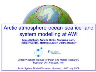
Arctic atmosphere-ocean-sea ice-land system modelling at AWI Klaus Dethloff , Annette Rinke, Wolfgang Dorn, Rüdiger Gerdes, Matthias Läuter, Dörthe Handorf Alfred Wegener Institute for Polar- and Marine Research, Research Unit Potsdam, AWI

E N D
Arctic atmosphere-ocean-sea ice-land system modelling at AWI Klaus Dethloff, Annette Rinke, Wolfgang Dorn, Rüdiger Gerdes, Matthias Läuter, Dörthe Handorf Alfred Wegener Institute for Polar- and Marine Research, Research Unit Potsdam, AWI Arctic System Model Workshop Montreal, 16-17 July 2009
This talk: • Motivation • Atmospheric RCM • Coupled A-O-I RCM • Coupled A-L-S RCM • Regionally focused global model
O O O The Arctic in the global Earth system Clouds Ozone Aerosols CH4 H Run-off Sea ice CO2 H Water Heat L Momentum Process studies, Regional and Global Earth System Models • RCM as magnifying glass due to higher resolution • Reduction of uncertainties in attribution of current climate changes • Improved climate model projections for next IPPC Report Tracer H
Regional climate model, Arctic integration areaHigh horizontal resolution of regional topographic structures at the surface, Improved simulation of hydrodynamical instabilities and baroclinic cyclones (m) RCM HIRHAM, 50 km GCM (ERA40) Initial & boundary conditions for the RCM provided by ERA-40 data
This talk: • Motivation • Atmospheric RCM • Coupled A-O-I RCM • Coupled A-L-S RCM • Regionally focused global model
North Pole drifting station NP 35 NP35: North Pole drifting station No. 35 operated by AARI St. Petersburg from October 2007 until July 2008 Contribution to IPY Atmospheric observations: Radiosonde (up to 30 km) (twice every day, at noon and midnight) Tethered balloon (lowest 500 m) (if weather conditions allowed it, at 55 days) Synoptic weather recording (at surface) (four times per day, every 6 hours)
Regional atmospheric climate model simulations Trajectory of NP35 ice camp November 2007-March 2008 HIRHAMregional climate model Pan Arctic domain, 110x100 grid points 50 km horizontal resolution 25 vertical levels (lowest level at 10 m, 10 levels in lowest 1 km) boundary forcing by ECMWF operational analyses
Regional atmospheric climate model simulations to compare with NP35 data set How to compare simulation output with single point observations? Regional climate model simulations with 2 different setups: 1) HIRHAM in forecast mode - simulation with initialization every 12 hours 2) HIRHAM in climate mode with ensemble approach - initialization only at the beginning of the month - series of simulations with slightly different initial conditions - 5 ensemble members (ctrl, ±6 and ±12 hours initial state) - ensemble mean & across-ensemble member scatter
Temperature [°C] Temperature [°C] Meteorological evolution at NP35 during February 2008 -evolution of temperature profile in simulations - Observation HIRHAM Climate Ensemble mean Temperature [°C] Pressure [hPa] Pressure [hPa] HIRHAM Forecast12 HIRHAM Bias Temperature bias [°C] HIRHAM F12 - Obs Pressure [hPa] Pressure [hPa] Stable PBL
This talk: • Motivation • Atmospheric RCM • Coupled A-O-I RCM • Coupled A-L-S RCM • Regionally focused global model
Coupled regional Atmosphere-Ocean-Sea Ice Model High horizontal resolution of regional topographic structures at the surface, Improved simulation of hydro-dynamical instabilities and baroclinic cyclones Sea ice is an integrator of oceanic and atmospheric changes • Atmosphere modelHIRHAM • parallelized version • 110×100 grid points • horizontal resolution 0.5° • 19 vertical levels • Ocean–ice modelNAOSIM • based on MOM-2 • Elastic-Viscous Plastic ice dynamics • 242×169 grid points • horizontal resolution 0.25° • 30 vertical levels • Boundary forcing ERA-40
Simulation of sea ice concentration anomaly of September 1998 over the Beaufort sea (SSMI and 12 year long simulations after spin up time of 7 years) Coupled RCM Sea ice anomaly in Beaufort Sea well simulated by the coupled model Atmospheric circulation Anticyclonic flow in the Beaufort Sea Ice growth parameterization during winter Influence on simulated sea ice Ice albedo parameterization crucial factor for ice melting during summer SSMI: Special Sensor Microwave Imager
Standard deviation of sea ice concentration (%) in September 1988-2000, spin up time: 1980-1987 Dorn et al. OASJ 2008 Satellite observations Coupled Arctic climate model Importance of internal variability due to atmospheric processes
Differences in September sea level pressure (hPa) and ice drift vectors (June-September) between “high-ice” minus “low-ice” years (1988-2000) High-ice years are 1996, 1988, 1992, and 1994 in the observation and 1989, 1996, 1988, and 1997 in simulation, Low-ice years are 1995, 1990, 1999, and 2000 in the observation and 1992, 1999, 1993, and 1991 in simulation. Cyclonic ice drift pattern during high-ice years Anticyclonic ice drift pattern during low-ice years Strong influence of summertime atmospheric circulation on sea ice drift. Dorn et al. , OASJ, 2, 2008
Arctic Sea-Ice Extent, Dec. 1997-1998, Sensitivity Experiments Already after one year there are model deviations in ice volume of up to 4500 km3 (one third of the total volume) as a result of altered sea ice- snow albedo parameterizations.
A-O-I RCM Combination of improved parameterizations for ice growth, sea ice albedo and snow cover improves the simulation of summer sea ice. Dorn et al., JGR, 2007, OASJ 2008, OM 2009. Change from HIRHAM 4 to HIRHAM 5 using the ECHAM 5 physical parameterizations New formulation of long-wave radiation and cloud physics. Long term simulations up to the year 2008/09 with NCEP and ERA boundary forcing and validation using recent measurements on NP 35 and NP 36 in progress.
This talk: • Motivation • Atmospheric RCM • Coupled A-O-I RCM • Coupled A-L-S RCM • Regionally focused global model
Coupled atmosphere-land surface-soil model • An important component of the climate and environmental system poorly represented in RCMs • characteristics of land surface (e.g., roughness, albedo, emissivity, soil texture, vegetation type, snow and ice cover extent, leaf area index, and seasonality) • states of soil properties over land (e.g., soil moisture, soil temperature, canopy temperature, snow water equivalent) exchanges of momentum, energy, water vapour, and trace gases between land surface, soil and the overlying atmosphere
A-L-S RCM • Coupled atmosphere- • land surface-soil • model • horiz. resolution • 0.25° or 0.5° • Atmosphere • ECHAM4 parameterizations • 19 vertical levels • Land surface-soil • LSM module from NCAR • 6 layers • (total depth of 6 m) Topography (m)
Forest Forest tundra Non-wood tundra 0-10 cm peat 0-10 cm moss/lichen 0-10 cm moss 10-30 cm peat Modified land surface model Inclusion of a soil organic layer Original LSM ground column treated as mineral ground texture (sand, silt, clay) 1) Moss, peat, lichen are included as 3 additional texture types thermal and hydraulic parameters are specified according to Beringer et al. (2001), 30 times lower thermal conductivity, 10 times higher hydraulic parameters 2) different textures are specified for each layer Top organic layer prescribed according to 3 land surface types in model domain
A-L-S RCM Sensitivity of Arctic climate simulation to a soil organic layer 21-year-long run 1979-1999 driven by ERA-40. Different land surface types in RCM describe fractional cover of plant types influence surface fluxes Top organic layer has been prescribed according to land types: ° only mineral soil texture (orig. model) “CTRL” ° top soil organic layer included “SOL” first 11 years neglected: spin-up time of deep ground conditions 10 years (1990-1999) are analyzed Climatic effect of soil layer “SOL minus CTRL” Forest Tundra Non-Wood Tundra Forest Rinke et al., GRL 2008
SLP bias (GCM composite minus ERA40), 1981-2000, 14 GCMs (Chapman & Walsh, 2007) [hPa] Changes in atmosphere (“SOL minus CTRL”), Winter Top organic layer reduces ground soil temperatures by 0.5 ° C up to 8 °C Changes in the surface heat fluxes affects regional atmospheric circulation 2m air temperature [K] Sea level pressure (hPa) Remote influences due to soil properties Reduction of GCM bias in the Arctic.
This talk: • Motivation • Atmospheric RCM • Coupled A-O-I RCM • Coupled A-L-S RCM • Regionally focused global model
Atmospheric dynamical core on unstructured triangular grids Shallow water model Describe two-way dynamical feedbacks between regions with high and low horizontal resolution Arctic and rest of globe • Adaptive triangular grid • Spherical geometry and spherical • triangular coordinates • Feedbacks between planetary • and synoptic-scale waves • Approximation of curvature of the finite • elements in space by polynomial order k • Explicit Runge-Kutta time step
(S)-(R), Uniform Grid (S)-(R), Regionally resol. Grid Day 30 Two-way coupling between regional and global scales • Deviations in geopotential heights (gpm) from geostrop. • balanced field after 30 days due to orogr. perturbation • Reference simulation (R) without Greenland topography • Sensitivity simulation (S) with Greenland topography • Simulation with uniform grid Dx=133 km • Simulation with with regionally resolved grid Dx = 67 km Impact of the regionally resolved area on global circulation structures
Summary: • RCM results are sensitive to the choice of • the integration domain, • lateral and lower boundary conditions, • horizontal and vertical resolution, • parameterizations. • Regionally coupled models of the Arctic climate system and improved data sets can contribute to the attribution of ongoing changes. • Development of new ideas (e.g. sea ice albedo, organic top layer) for improving global models in the Arctic. • Two-way feedbacks has to be considered within a global model setup by regionally focused modelling of the area of interest.
Difference in atmosphere “HIRHAM-LSM minus HIRHAM” 1979-93, Saha et al. (2006) Summer (JJA) Winter (DJF) [Pa] [Pa] Mean sea level pressure (Pa) and 10m wind (m/s) Remote influences
Standard deviation (°C) of surface air temperature, winter (1958-2001), Matthes et al., 2009, submitted ERA-40 RCM HIR_LSM °C Atmosphere-surface-soil feedbacks Impacts over Siberia and Alaska
New soil scheme from Land Surface Model LSM (NCAR) Old soil scheme ECHAM4 (Roeckner et al., 1996) with a soil moisture bucket model atmospheric radiative + turbulent fluxes at the surface precipitation + evaporation Tstemperature at the interface between atmosphere and surface Vegetation runoff Snow Layer 1, dz=0.10 m Thawing & Freezing Layer 2, dz=0.20 m Layer 3, dz=0.40 m Conservation equation to calculate soil water content WSsoil (z) Heat conduction equation to calculate Tsoil (z) Layer 4, dz=0.80 m Layer 5, dz=1.60 m Layer 6, dz=3.20 m 6.30 m
k 2 4 6 8 Atmospheric shallow-water modelInfluence of horizontal resolution on normalised model error • Hyperbolic system for layer depth, momentum • Spherical geometry and spherical triangular coordinates • Polynomial order k approximation of curvature of the finite elements in space • Polynomial degree k convergence order k+1 Test case: Barotropic instability of a geostrophic jet at 30 ° N
September sea level pressure (hPa) for “high-ice” and “low-ice” years within 1988-2000 in ERA-40 and CRCM L L High ice cover low sea level pressure cyclonic conditions More ice transport into the Beaufort Sea more sea ice to the Laptev Sea Weaker transpolar drift weaker sea ice outflow through Fram Strait H H Low ice cover high sea level pressure anticyclonic conditions Stronger transpolar drift Sea ice export through the Fram Strait
Atmospheric circulation February 2008 ECMWF Sea level pressure (hPa; color) 500 hPa geopotential height (m; isoline) X X Position of NP 35 in February 2008 HIRHAM Climate Ensemble mean HIRHAM Forecast12 X X
Land-surface-soil and PBL turbulence closure Atmosphere Surface layer energy budget: Rn Radiative fluxes H0 Heat fluxes E0 Humidity fluxes Hm Ground heat fluxes compute surface fluxes and update surface temperature and humidity by solving soil model and surface energy budget Soil
Day 3 Vorticity, Jet stream Day 6 • Zonal wind jet with initial perturbation • Regulär grid Dx = 30 km • Development of filaments • Meridional mixing Multiple scale interaction: Barotropic instability Läuter et al., J. Computational Physics 2008