An Introduction to Light Fields
200 likes | 351 Vues
An Introduction to Light Fields. Mel Slater. Outline. Introduction Rendering Representing Light Fields Practical Issues Conclusions. Introduction. L(p, ) is defined over the set of all all rays (p, ) with origins at points on surfaces Domain of L is 5D ray space.

An Introduction to Light Fields
E N D
Presentation Transcript
An Introduction to Light Fields Mel Slater
Outline • Introduction • Rendering • Representing Light Fields • Practical Issues • Conclusions
Introduction • L(p, ) is defined over the set of all all rays (p, ) with origins at points on surfaces • Domain of L is 5D ray space. • L is constant in ‘free space’, space free of occluders: ray occluded ray in ‘free space’
Introduction: Free Space • Radiance is constant along each ray in free space emanating from the convex hull around the scene
Introduction: Restrict L to 4D • In free space the domain of L can be restricted to 4D • L(s,t,u,v) can represent all rays between two parallel planes – a ‘light slab’. uv plane Here radiance isflowing in directionuv to st. st plane
Introduction:Light Field = 6 Light Slabs • 6 light slabs can represent rays in all directions: • Near-far, Far-near • Left-right, Right-left • Bottom-top, Top-bottom • Discretisation provides approximation to ‘all rays’.
Introduction:Assigning Radiance to Each Ray Image plane uv plane st plane cop • Place the cop at each grid point on st plane • Use uv plane as an image plane. • Each ray is assigned a radiance.
Introduction:Synthesising a New Image u0 u1 u2 u3 u4 Image plane uv plane st plane s0 s1 s2 s3 s4 New image plane The image ray is approximated By L(s3, u1) cop
Introduction: Summary • Light field is a discrete representation of L restricted to the 4D free space domain. • It relies on production of a large set of images under strict viewing conditions. • Most often used for virtual images of real scenes – based on digital photographs. • Can be used for synthetic scenes – not much point unless globally illuminated • Supports real-time walkthrough of scenes.
Rendering • Each st grid-point is associated with a uv image v t u Let a texture map consistingof the image be associated with st grid-point. s
Rendering: Texture Mapping • Each st grid-point square is projected to the uv plane v a b t d c u The st square is renderedwith the texture map and texture coords abcd cop s
Rendering: Quadrilinear Interpolation • Perform linear interpolation on s • Repeat expansion for t,u,v. v1 (u,v) v0 u0 u1 t1 (s,t) t0 s0 s1 L(s,t0,u0,v0)= 0L(s0,t0,u0,v0)+ 1L(s1,t0,u0,v0)
Efficient Rendering: Linear-Bilinear Interpolation • Gortler shows that texture mapping cannot be used to reproduce quadrilinear interpolation, but linear (on st), bilinear (on uv). For the grid-point Prender each of the triangles ABP, BCP, CDP, DEP, EFP,FAP with alpha-blending and texture mapping: =1 at P and =0 at each vertex. B C D A P(s,t) F E
Rendering: Depth Correction • Use approximate polygon mesh to provide depth information. u0 u1 u2 u3 u4 Normally s1 u4 wouldbe used to approximate viewing ray. s1 u3 is more accurate. object surface s0 s1 s2 cop
Representation • The 2PP has many computational advantages: • Efficient representation of images • Texture mapping hardware used for rendering • Linear properties of the representation. • It is not a ‘uniform’ representation • As the viewpoint moves so the density and distribution of close-by rays will change, and thus image quality will change during walkthrough.
Representation: Using Spheres • Camahort and Fussel, 1999 carried out study of 3 representations: • 2PP – 2-plane • 2SP – 2-sphere • DPP – direction and point DPP theoretically shown to introduceless sampling bias, greater uniformity.
Practical Issues • Idea placement of st and uv planes? • st outside the scene, and uv ideally through ‘centre’ of scene. • Ideally uv grid-points as close as possible to scene geometry • Implication is that scenes with large depth range cannot be adequately represented.
Practical Issues: Resolution • What resolution should be used for st, uv? • st (MM) can afford to be sampled at lower rate, since the accuracy depends on uv (N N), close to scene surfaces. • Typical values are M=32, N=256 • for synthesis of 256 256 resolution images
Practical Issues: Memory • Suppose N=256, M=32 • Each light slab requires 28 28 25 25 =226 rays • Each ray carries 3Bytes (RGB) • There are 6 light slabs. • Full representation therefore requires: • 6 3 226 > 1Gb memory. • Compression scheme needed (vector quantization used in practice).
Conclusions • LF approach offers a different paradigm with many disadvantages, but interesting possibilities: • Exploits current hardware for a brute-force ‘solution’ of radiance equation. • Image of real scenes or synthetic scenes (and combinations). • Rendering time independent of scene complexity. • Promise of real-time walkthrough for global illumination