Chapter 9: Control Systems
Chapter 9: Control Systems. Control System. Control physical system’s output By setting physical system’s input Tracking E.g. Cruise control Thermostat control Disk drive control Aircraft altitude control Difficulty due to Disturbance: wind, road, tire, brake; opening/closing door…

Chapter 9: Control Systems
E N D
Presentation Transcript
Control System • Control physical system’s output • By setting physical system’s input • Tracking • E.g. • Cruise control • Thermostat control • Disk drive control • Aircraft altitude control • Difficulty due to • Disturbance: wind, road, tire, brake; opening/closing door… • Human interface: feel good, feel right…
Open-Loop Control Systems • Plant • Physical system to be controlled • Car, plane, disk, heater,… • Actuator • Device to control the plant • Throttle, wing flap, disk motor,… • Controller • Designed product to control the plant
Open-Loop Control Systems • Output • The aspect of the physical system we are interested in • Speed, disk location, temperature • Reference • The value we want to see at output • Desired speed, desired location, desired temperature • Disturbance • Uncontrollable input to the plant imposed by environment • Wind, bumping the disk drive, door opening
Other Characteristics of open loop • Feed-forward control • Delay in actual change of the output • Controller doesn’t know how well thing goes • Simple • Best use for predictable systems
Close Loop Control Systems • Sensor • Measure the plant output • Error detector • Detect Error • Feedback control systems • Minimize tracking error
Designing Open Loop Control System • Develop a model of the plant • Develop a controller • Analyze the controller • Consider Disturbance • Determine Performance • Example: Open Loop Cruise Control System
Model of the Plant • May not be necessary • Can be done through experimenting and tuning • But, • Can make it easier to design • May be useful for deriving the controller • Example: throttle that goes from 0 to 45 degree • On flat surface at 50 mph, open the throttle to 40 degree • Wait 1 “time unit” • Measure the speed, let’s say 55 mph • Then the following equation satisfy the above scenario • vt+1=0.7*vt+0.5*ut • 55 = 0.7*50+0.5*40 • IF the equation holds for all other scenario • Then we have a model of the plant
Designing the Controller • Assuming we want to use a simple linear function • ut=F(rt)= P * rt • rt is the desired speed • Linear proportional controller • vt+1=0.7*vt+0.5*ut = 0.7*vt+0.5P*rt • Let vt+1=vt at steady state = vss • vss=0.7*vss+0.5P*rt • At steady state, we want vss=rt • P=0.6 • I.e. ut=0.6*rt
Analyzing the Controller • Let v0=20mph, r0=50mph • vt+1=0.7*vt+0.5(0.6)*rt =0.7*vt+0.3*50= 0.7*vt+15 • Throttle position is 0.6*50=30 degree
Considering the Disturbance • Assume road grade can affect the speed • From –5mph to +5 mph • vt+1=0.7*vt+10 • vt+1=0.7*vt+20
Determining Performance • Vt+1=0.7*vt+0.5P*r0-w0 • v1=0.7*v0+0.5P*r0-w0 • v2=0.7*(0.7*v0+0.5P*r0-w0)+0.5P*r0-w0 =0.7*0.7*v0+(0.7+1.0)*0.5P*r0-(0.7+1.0)w0 • vt=0.7t*v0+(0.7t-1+0.7t-2+…+0.7+1.0)(0.5P*r0-w0) • Coefficient of vt determines rate of decay of v0 • >1 or <-1, vt will grow without bound • <0, vt will oscillate
Stability • ut = P * (rt-vt) • vt+1 = 0.7vt+0.5ut-wt = 0.7vt+0.5P*(rt-vt)-w =(0.7-0.5P)*vt+0.5P*rt-wt • vt=(0.7-0.5P)t*v0+((0.7-0.5P)t-1+(0.7-0.5P)t-2+…+0.7-0.5P+1.0)(0.5P*r0-w0) • Stability constraint (I.e. convergence) requires |0.7-0.5P|<1 -1<0.7-0.5P<1 -0.6<P<3.4
Reducing effect of v0 • ut = P * (rt-vt) • vt+1 = 0.7vt+0.5ut-wt = 0.7vt+0.5P*(rt-vt)-w =(0.7-0.5P)*vt+0.5P*rt-wt • vt=(0.7-0.5P)t*v0+((0.7-0.5P)t-1+(0.7-0.5P)t-2+…+0.7-0.5P+1.0)(0.5P*r0-w0) • To reduce the effect of initial condition • 0.7-0.5P as small as possible • P=1.4
Avoid Oscillation • ut = P * (rt-vt) • vt+1 = 0.7vt+0.5ut-wt = 0.7vt+0.5P*(rt-vt)-w =(0.7-0.5P)*vt+0.5P*rt-wt • vt=(0.7-0.5P)t*v0+((0.7-0.5P)t-1+(0.7-0.5P)t-2+…+0.7-0.5P+1.0)(0.5P*r0-w0) • To avoid oscillation • 0.7-0.5P >=0 • P<=1.4
Perfect Tracking • ut = P * (rt-vt) • vt+1 = 0.7vt+0.5ut-wt = 0.7vt+0.5P*(rt-vt)-w =(0.7-0.5P)*vt+0.5P*rt-wt • vss=(0.7-0.5P)*vss+0.5P*r0-w0 (1-0.7+0.5P)vss=0.5P*r0-w0 vss=(0.5P/(0.3+0.5P)) * r0 - (1.0/(0.3+0.5P)) * wo • To make vss as close to r0 as possible • P should be as large as possible
Close-Loop Design • ut = P * (rt-vt) • Finally, setting P=3.3 • Stable, track well, some oscillation • ut = 3.3 * (rt-vt)
Analyze the controller • v0=20 mph, r0=50 mph, w=0 • vt+1 = 0.7vt+0.5P*(rt-vt)-w = 0.7vt+0.5*3.3*(50-vt) • ut = P * (rt-vt) = 3.3 * (50-vt) • But ut range from 0-45 • Controller saturates
Analyze the controller • v0=20 mph, r0=50 mph, w=0 • vt+1 = 0.7vt+0.5*ut • ut = 3.3 * (50-vt) • Saturate at 0, 45 • Oscillation! • “feel bad”
Analyze the controller • Set P=1.0 to void oscillation • Terrible SS performance
Minimize the effect of disturbance • vt+1 = 0.7vt+0.5*3.3*(rt-vt)-w • w=-5 or +5 • 39.74 • Close to 42.31 • Better than • 33 • 66 • Cost • SS error • oscillation
General Control System • Objective • Causing output to track a reference even in the presence of • Measurement noise • Model error • Disturbances • Metrics • Stability • Output remains bounded • Performance • How well an output tracks the reference • Disturbance rejection • Robustness • Ability to tolerate modeling error of the plant
Performance (generally speaking) • Rise time • Time it takes form 10% to 90% • Peak time • Overshoot • Percentage by which Peak exceed final value • Settling time • Time it takes to reach 1% of final value
Plant modeling is difficult • May need to be done first • Plant is usually on continuous time • Not discrete time • E.g. car speed continuously react to throttle position, not at discrete interval • Sampling period must be chosen carefully • To make sure “nothing interesting” happen in between • I.e. small enough • Plant is usually non-linear • E.g. shock absorber response may need to be 8th order differential • Iterative development of the plant model and controller • Have a plant model that is “good enough”
Controller Design: P • Proportional controller • A controller that multiplies the tracking error by a constant • ut = P * (rt-vt) • Close loop model with a linear plant • E.g. vt+1 = (0.7-0.5P)*vt+0.5P*rt-wt • P affects • Transient response • Stability, oscillation • Steady state tacking • As large as possible • Disturbance rejection • As large as possible
Controller Design: PD • Proportional and Derivative control • ut = P * (rt-vt) + D * ((rt-vt)-(rt-1-vt-1)) = P * et+ D * (et-et-1) • Consider the size of error over time • Intuitively • Want to “push” more if the error is not reducing fast enough • Want to “push” less if the error is reducing really fast
PD Controller • Need to keep track of error derivative • E.g. Cruise controller example • vt+1 = 0.7vt+0.5ut-wt • Let ut = P * et + D * (et-et-1), et=rt-vt • vt+1=0.7vt+0.5*(P*(rt-vt)+D*((rt-vt)-(rt-1-vt-1)))-wt • vt+1=(0.7-0.5*(P+D))*vt+0.5D*vt-1+0.5*(P+D)*rt-0.5D*rt-1-wt • Assume reference input and distribance are constant, the steady-state speed is • Vss=(0.5P/(1-0.7+0.5P)) * r • Does not depend on D!!! • P can be set for best tracking and disturbance control • Then D set to control oscillation/overshoot/rate of convergence
PI Control • Proportional plus integral control • ut=P*et+I*(e0+e1+…+et) • Sum up error over time • Ensure reaching desired output, eventually • vss will not be reached until ess=0 • Use P to control disturbance • Use I to ensure steady state convergence and convergence rate
PID Controller • Combine Proportional, integral, and derivative control • ut=P*et+I*(e0+e1+…+et)+D*(et-et-1) • Available off-the shelf
Software Coding • Main function loops forever, during each iteration • Read plant output sensor • May require A2D • Read current desired reference input • Call PidUpdate, to determine actuator value • Set actuator value • May require D2A
Software Coding (continue) • Pgain, Dgain, Igain are constants • sensor_value_previous • For D control • error_sum • For I control
Computation • ut=P*et+I*(e0+e1+…+et)+D*(et-et-1)
PID tuning • Analytically deriving P, I, D may not be possible • E.g. plant not is not available, or to costly to obtain • Ad hoc method for getting “reasonable” P, I, D • Start with a small P, I=D=0 • Increase D, until seeing oscillation • Reduce D a bit • Increase P, until seeing oscillation • Reduce D a bit • Increase I, until seeing oscillation • Iterate until can change anything without excessive oscillation
Practical Issues with Computer-Based Control • Quantization • Overflow • Aliasing • Computation Delay
Quantization & Overflow • Quantization • Can’t store 0.36 as 4-bit fractional number • Can only store 0.75, 0.59, 0.25, 0.00, -0.25, -050,-0.75, -1.00 • Choose 0.25 • Result in quantization error of 0.11 • Sources of quantization error • Operations, e.g. 0.50*0.25=0.125 • Can use more bits until input/output to the environment/memory • A2D converters • Overflow • Can’t store 0.75+0.50 = 1.25 as 4-bit fractional number • Solutions: • Use fix-point representation/operations carefully • Time-consuming • Use floating-point co-processor • Costly
Aliasing • Quantization/overflow • Due to discrete nature of computer data • Aliasing • Due to discrete nature of sampling
Aliasing Example • Sampling at 2.5 Hz, period of 0.4, the following are indistinguishable • y(t)=1.0*sin(6πt), frequency 3 Hz • y(t)=1.0*sin(πt), frequency of 0.5 Hz • In fact, with sampling frequency of 2.5 Hz • Can only correctly sample signal below Nyquist frequency 2.5/2 = 1.25 Hz
Computation Delay • Inherent delay in processing • Actuation occurs later than expected • Need to characterize implementation delay to make sure it is negligible • Hardware delay is usually easy to characterize • Synchronous design • Software delay is harder to predict • Should organize code carefully so delay is predictable and minimized • Write software with predictable timing behavior (be like hardware) • Time Trigger Architecture • Synchronous Software Language
Benefit of Computer Control • Cost!!! • Expensive to make analog control immune to • Age, temperature, manufacturing error • Computer control replace complex analog hardware with complex code • Programmability!!! • Computer Control can be “upgraded” • Change in control mode, gain, are easy to do • Computer Control can be adaptive to change in plant • Due to age, temperature, …etc • “future-proof” • Easily adapt to change in standards,..etc