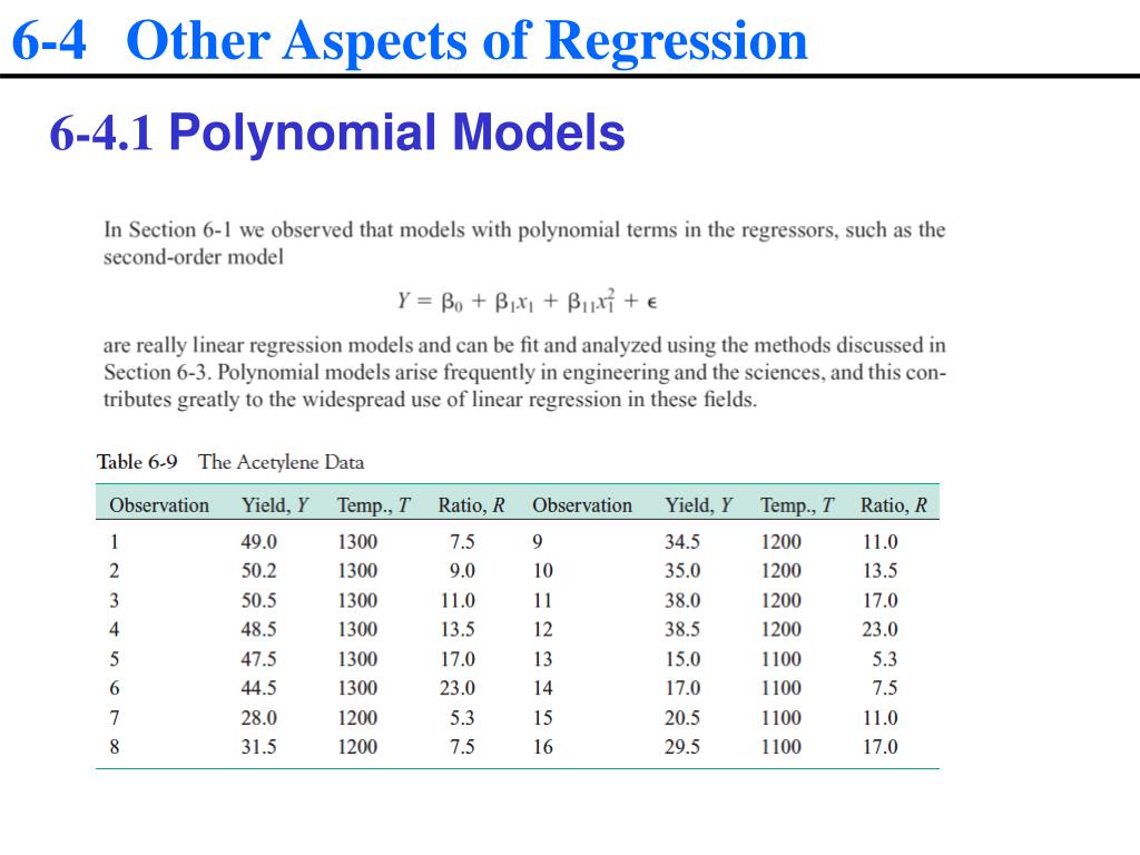
6-4 Other Aspects of Regression. 6-4.1 Polynomial Models. 6-4 Other Aspects of Regression. 6-4.1 Polynomial Models. 6-4 Other Aspects of Regression. 6-4.1 Polynomial Models.
Une image / un lien ci-dessous est fourni (tel quel) pour télécharger la présentation
Politique de téléchargement : le contenu du site vous est fourni TEL QUEL pour votre information et votre usage personnel ; il ne peut être vendu, concédé sous licence ni partagé sur d’autres sites sans l’accord de son auteur.Le contenu vous est fourni TEL QUEL, pour votre information et votre usage personnel uniquement.Téléchargez la présentation en cliquant sur ce lien.Lors du téléchargement, si vous ne parvenez pas à télécharger une présentation, l’éditeur a peut-être supprimé le fichier de son serveur.Pendant le téléchargement, si vous ne parvenez pas à obtenir une présentation, le fichier a peut-être été supprimé par l’éditeur.
6-4 Other Aspects of Regression 6-4.1 Polynomial Models Suppose that we wanted to test the contribution of the second-order terms to this model. In other words, what is the value of expanding the model to include the additional terms?
6-4 Other Aspects of Regression LINEAR REGRESSION MODEL - REDUCED MODEL The REG Procedure Model: MODEL1 Dependent Variable: YIELD Number of Observations Read 16 Number of Observations Used 16 Analysis of Variance Sum of Mean Source DF Squares Square F Value Pr > F Model 2 1952.97853 976.48926 74.35 <.0001 Error 13 170.73085 13.13314 Corrected Total 15 2123.70937 Root MSE 3.62397 R-Square 0.9196 Dependent Mean 36.10625 Adj R-Sq 0.9072 CoeffVar 10.03695 Parameter Estimates Parameter Standard Variance Variable DF Estimate Error t Value Pr > |t| Inflation Intercept 1 36.10634 0.90599 39.85 <.0001 0 TEMPC 1 0.13396 0.01191 11.25 <.0001 1.05264 RATIOC 1 0.35106 0.16955 2.07 0.0589 1.05264
6-4 Other Aspects of Regression 6-4.1 Polynomial Models where: SSER = SSE for Reduced Model SSEF= SSE for Full Model = number of ’s in H0 For given , we reject H0 if: Partial F>tabled F with dof = , numerator , denominator
6-4 Other Aspects of Regression Example OPTIONS NOOVP NODATE NONUMBER; DATA BIDS; INFILE 'C:\users\myung\Documents\Teaching\학부과목\imen214-stats\bids.dat'; INPUT PRICE QUANTITY BIDS; LOGPRICE=LOG(PRICE); QUANSQ=QUANTITY**2; PROCREG DATA=BIDS; MODEL PRICE= QUANTITY/P CLM CLI XPX; PLOT PRICE*QUANTITY/PRED CONF; /* SCATTER PLOT */ PLOT R.*P.; TITLE 'LINEAR REGRESSION OF PRICE VS. QUANTITY'; PROCREG DATA=BIDS; MODEL LOGPRICE= QUANTITY/P CLM CLI XPX; PLOT LOGPRICE*QUANTITY/PRED CONF; /* SCATTER PLOT */ PLOT R.*P.; TITLE 'LINEAR REGRESSION OF LOGPRICE VS. QUANTITY'; PROCREG DATA=BIDS; MODEL PRICE= QUANTITY QUANSQ/P CLM CLI XPX; PLOT PRICE*QUANTITY; /* SCATTER PLOT */ PLOT R.*P.; TITLE 'QUADRATIC REGRESSION OF PRICE VS. QUANTITY'; RUN; QUIT;
6-4 Other Aspects of Regression LINEAR REGRESSION OF PRICE VS. QUANTITY The REG Procedure Model: MODEL1 Model Crossproducts X'X X'Y Y'Y Variable Intercept QUANTITY PRICE Intercept 30 273 2374.97 QUANTITY 273 3688.98 12492.46 PRICE 2374.97 12492.46 266887.1815 --------------------------------------------------------------------------------------------- LINEAR REGRESSION OF PRICE VS. QUANTITY The REG Procedure Model: MODEL1 Dependent Variable: PRICE Number of Observations Read 30 Number of Observations Used 30 Analysis of Variance Sum of Mean Source DF Squares Square F Value Pr > F Model 1 69039 69039 196.62 <.0001 Error 28 9831.89259 351.13902 Corrected Total 29 78871 Root MSE 18.73870 R-Square 0.8753 Dependent Mean 79.16567 Adj R-Sq 0.8709 CoeffVar 23.67024 Parameter Estimates Parameter Standard Variable DF Estimate Error t Value Pr > |t| Intercept 1 148.05523 5.98682 24.73 <.0001 QUANTITY 1 -7.57028 0.53989 -14.02 <.0001
6-4 Other Aspects of Regression LINEAR REGRESSION OF LOGPRICE VS. QUANTITY The REG Procedure Model: MODEL1 Model Crossproducts X'X X'Y Y'Y Variable Intercept QUANTITY LOGPRICE Intercept 30 273 123.86106074 QUANTITY 273 3688.98 990.08475122 LOGPRICE 123.86106074 990.08475122 527.52302023 --------------------------------------------------------------------------------------------- LINEAR REGRESSION OF LOGPRICE VS. QUANTITY The REG Procedure Model: MODEL1 Dependent Variable: LOGPRICE Number of Observations Read 30 Number of Observations Used 30 Analysis of Variance Sum of Mean Source DF Squares Square F Value Pr > F Model 1 15.59165 15.59165 799.63 <.0001 Error 28 0.54596 0.01950 Corrected Total 29 16.13761 Root MSE 0.13964 R-Square 0.9662 Dependent Mean 4.12870 Adj R-Sq 0.9650 CoeffVar 3.38210 Parameter Estimates Parameter Standard Variable DF Estimate Error t Value Pr > |t| Intercept 1 5.16397 0.04461 115.75 <.0001 QUANTITY 1 -0.11377 0.00402 -28.28 <.0001
6-4 Other Aspects of Regression 6-4.2 Categorical Regressors • Many problems may involve qualitative or categorical variables. • The usual method for the different levels of a qualitative variable is to use indicator variables. • For example, to introduce the effect of two different operators into a regression model, we could define an indicator variable as follows:
6-4 Other Aspects of Regression Example 6-10 Y=gas mileage, x1=engine displacement, x2=horse power x3=0 if automatic transmission 1 if manual transmission if automatic (x3=0), then if manual (x3=1), then +)+ It is unreasonable because x1, x2 effects to x3 are not involved in the model Interaction model: if automatic (x3=0), then if manual (x3=1), then
6-4 Other Aspects of Regression Dummy Variables Many times a qualitative variable seems to be needed in a regression model. This can be accomplished by creating dummy variables or indicator variables. If a qualitative variable has levels you will need dummy variables. Notice that in ANOVA if a treatment had levels it had degrees of freedom. The ith dummy variable is defined as This can be done automatically in PROC GLM by using the CLASSS statement as we did in ANOVA. Any dummy variables defined with respect to a qualitative variable must be treated as a group. Individual t-tests are not meaningful. Partial F-tests must be performed on the group of dummy variables.
6-4 Other Aspects of Regression MODEL WITH DUMMY VARIABLE The REG Procedure Model: MODEL1 Dependent Variable: QUALITY Number of Observations Read 24 Number of Observations Used 24 Analysis of Variance Sum of Mean Source DF Squares Square F Value Pr > F Model 3 339.74858 113.24953 23.05 <.0001 Error 20 98.25142 4.91257 Corrected Total 23 438.00000 Root MSE 2.21643 R-Square 0.7757 Dependent Mean 84.50000 Adj R-Sq 0.7420 CoeffVar 2.62300 Parameter Estimates Parameter Standard Variable DF Estimate Error t Value Pr > |t| Intercept 1 89.80615 2.99018 30.03 <.0001 FORM 1 1.81923 0.32599 5.58 <.0001 RESIDUE 1 -3.37945 0.68582 -4.93 <.0001 REGION1 1 -3.40619 0.91941 -3.70 0.0014
6-4 Other Aspects of Regression INTERACTION MODEL WITH DUMMY VARIABLE The REG Procedure Model: MODEL1 Dependent Variable: QUALITY Number of Observations Read 24 Number of Observations Used 24 Analysis of Variance Sum of Mean Source DF Squares Square F Value Pr > F Model 5 342.36626 68.47325 12.89 <.0001 Error 18 95.63374 5.31299 Corrected Total 23 438.00000 Root MSE 2.30499 R-Square 0.7817 Dependent Mean 84.50000 Adj R-Sq 0.7210 CoeffVar 2.72780 Parameter Estimates Parameter Standard Variable DF Estimate Error t Value Pr > |t| Intercept 1 88.25694 4.83957 18.24 <.0001 FORM 1 1.98252 0.42919 4.62 0.0002 RESIDUE 1 -3.21529 0.95251 -3.38 0.0034 REGION1 1 -1.70670 6.57164 -0.26 0.7980 FR 1 -0.64190 0.94343 -0.68 0.5049 RR 1 0.43032 1.89360 0.23 0.8228
6-4 Other Aspects of Regression Example OPTIONSNOOVPNODATENONUMBER; DATA appraise; INPUT price units age size parking area cond$ @@; IF COND='F'THEN COND1=1; ELSE COND1=0; IF COND='G'THEN COND2=1; ELSE COND2=0; CARDS; 90300 4 82 4635 0 4266 F 384000 20 13 17798 0 14391 G 157500 5 66 5913 0 6615 G 676200 26 64 7750 6 34144 E 165000 5 55 5150 0 6120 G 300000 10 65 12506 0 14552 G 108750 4 82 7160 0 3040 G 276538 11 23 5120 0 7881 G 420000 20 18 11745 20 12600 G 950000 62 71 21000 3 39448 G 560000 26 74 11221 0 30000 G 268000 13 56 7818 13 8088 F 290000 9 76 4900 0 11315 E 173200 6 21 5424 6 4461 G 323650 11 24 11834 8 9000 G 162500 5 19 5246 5 3828 G 353500 20 62 11223 2 13680 F 134400 4 70 5834 0 4680 E 187000 8 19 9075 0 7392 G 93600 4 82 6864 0 3840 F 110000 4 50 4510 0 3092 G 573200 14 10 11192 0 23704 E 79300 4 82 7425 0 3876 F 272000 5 82 7500 0 9542 E PROCREGDATA=APPRAISE; MODEL PRICE=UNITS AGE AREA COND1 COND2/R; TITLE'REDUCED MODEL WITH DUMMY VARIABLE'; RUN; QUIT;
6-4 Other Aspects of Regression REDUCED MODEL WITH DUMMY VARIABLE The REG Procedure Model: MODEL1 Dependent Variable: price Number of Observations Read 24 Number of Observations Used 24 Analysis of Variance Sum of Mean Source DF Squares Square F Value Pr > F Model 5 1.040122E12 2.080244E11 253.02 <.0001 Error 18 14799036255 822168681 Corrected Total 23 1.054921E12 Root MSE 28673 R-Square 0.9860 Dependent Mean 296193 Adj R-Sq 0.9821 CoeffVar 9.68067 Parameter Estimates Parameter Standard Variable DF Estimate Error t Value Pr > |t| Intercept 1 176940 24044 7.36 <.0001 units 1 7256.44825 1185.16990 6.12 <.0001 age 1 -1155.95291 258.66820 -4.47 0.0003 area 1 11.86451 1.54837 7.66 <.0001 COND1 1 -61240 22434 -2.73 0.0138 COND2 1 -61572 18756 -3.28 0.0041
6-4 Other Aspects of Regression Analysisof Covariate Suppose we have the following setup. 3 2 3 2 3 4 2 2 3 Y 2 3 2 1 3 4 4 2 3 1 3 1 4 1 4 4 4 4 1 1 1 1 X Suppose X and Y are linearly related. We are interested in comparing the means of Y at the different levels of the treatment. Suppose a plot of the data looks like the following.
6-4 Other Aspects of Regression Why Use Covariates? Concomitant variables or covariates are used to adjust for factors that influence the Y measurements. In randomized block designs, we did the same thing, but there we could control the value of the block variable. Now we assume we can measure the variable, but not control it. The plot on the previous page demonstrates why we need covariates in some situations. If the covariate (X) was ignored we would most likely conclude that treatment level 3 resulted in a larger mean than 1 and 4 but not different from 2. If the linear relation is extended we see that the value of Y in level 3 could very well be less than that of 1, nearly equal to that of 4 and surely less than that of 2. One assumption we need, equivalent to the no interaction assumption in two-way ANOVA, is that the slopes of the linear relationship between X and Y is the same in each treatment level.
6-4 Other Aspects of Regression Checking for Equal Slopes The Model we fit first Treatment = 1 Y-intercept = slope= Treatment = r1 Y-intercept = slope= Treatment = r Y-intercept = slope= The test of equal slopes is If we fail to reject this we return the model without the interaction term and test without the interaction term and test
6-4 Other Aspects of Regression EXAMPLE Four different formulations of an industrial glue are being tested. The tensile strength of the glue is also related to the thickness. Five observations on strength (Y) and thickness (X) in 0.01 inches are obtained for each formulation. The data are shown in the following table.
6-4 Other Aspects of Regression Example OPTIONSNOOVPNODATENONUMBER; DATA GLUE; INPUT FORMULA STRENGTH THICK @@; CARDS; 1 46.5 13 1 45.9 14 1 49.8 12 1 46.1 12 1 44.3 14 2 48.7 12 2 49.0 10 2 50.1 11 2 48.5 12 2 45.2 14 3 46.3 15 3 47.1 14 3 48.9 11 3 48.2 11 3 50.3 10 4 44.7 16 4 43.0 15 4 51.0 10 4 48.1 12 4 48.6 11 PROCGLMDATA=GLUE; CLASS FORMULA; MODEL STRENGTH=FORMULA THICK FORMULA*THICK; OUTPUTOUT=OUT1 P=PRED R=RESID; TITLE'ANALYSIS OF COVARIANCE WITH INTERACTION'; PROCPLOTDATA=OUT1; PLOT STRENGTH*THICK=FORMULA; PLOT PRED*THICK=FORMULA; PLOT RESID*PRED=FORMULA; PROCGLMDATA=GLUE; CLASS FORMULA; MODEL STRENGTH=FORMULA THICK/SOLUTION; OUTPUTOUT=OUT2 P=PRED R=RESID; LSMEANS FORMULA/PDIFFSTDERR; TITLE'ANALYSIS OF COVARIANCE WITHOUT INTERACTION'; PROCPLOTDATA=OUT2; PLOT STRENGTH*THICK=FORMULA; PLOT PRED*THICK=FORMULA; PLOT RESID*PRED=FORMULA; RUN; QUIT;
6-4 Other Aspects of Regression ANALYSIS OF COVARIANCE WITH INTERACTION The GLM Procedure Dependent Variable: STRENGTH Sum of Source DF Squares Mean Square F Value Pr > F Model 7 74.01777794 10.57396828 7.22 0.0016 Error 12 17.56772206 1.46397684 Corrected Total 19 91.58550000 R-Square CoeffVar Root MSE STRENGTH Mean 0.808182 2.546457 1.209949 47.51500 Source DF Type I SS Mean Square F Value Pr > F FORMULA 3 11.05750000 3.68583333 2.52 0.1076 THICK 1 59.56576027 59.56576027 40.69 <.0001 THICK*FORMULA 3 3.39451766 1.13150589 0.77 0.5312 Source DF Type III SS Mean Square F Value Pr > F FORMULA 3 2.80437055 0.93479018 0.64 0.6046 THICK 1 41.34340945 41.34340945 28.24 0.0002 THICK*FORMULA 3 3.39451766 1.13150589 0.77 0.5312
6-4 Other Aspects of Regression ANALYSIS OF COVARIANCE WITHOUT INTERACTION The GLM Procedure Dependent Variable: STRENGTH Sum of Source DF Squares Mean Square F Value Pr > F Model 4 70.62326027 17.65581507 12.63 0.0001 Error 15 20.96223973 1.39748265 Corrected Total 19 91.58550000 R-Square CoeffVar Root MSE STRENGTH Mean 0.771118 2.487955 1.182152 47.51500 Source DF Type I SS Mean Square F Value Pr > F FORMULA 3 11.05750000 3.68583333 2.64 0.0876 THICK 1 59.56576027 59.56576027 42.62 <.0001 Source DF Type III SS Mean Square F Value Pr > F FORMULA 3 1.77104066 0.59034689 0.42 0.7397 THICK 1 59.56576027 59.56576027 42.62 <.0001 Standard Parameter Estimate Error t Value Pr > |t| Intercept 60.00712329 B 2.04941586 29.28 <.0001 FORMULA 1 -0.35801370 B 0.74829823 -0.48 0.6392 FORMULA 2 0.21006849 B 0.76349365 0.28 0.7870 FORMULA 3 0.47404110 B 0.75339742 0.63 0.5387 FORMULA 4 0.00000000 B . . . THICK -1.00993151 0.15469162 -6.53 <.0001 NOTE: The X'X matrix has been found to be singular, and a generalized inverse was used to solve the normal equations. Terms whose estimates are followed by the letter 'B' are not uniquely estimable.
6-4 Other Aspects of Regression ANALYSIS OF COVARIANCE WITHOUT INTERACTION The GLM Procedure Least Squares Means STRENGTH Standard LSMEAN FORMULA LSMEAN Error Pr > |t| Number 1 47.0754623 0.5354766 <.0001 1 2 47.6435445 0.5381512 <.0001 2 3 47.9075171 0.5300869 <.0001 3 4 47.4334760 0.5314395 <.0001 4 Least Squares Means for effect FORMULA Pr > |t| for H0: LSMean(i)=LSMean(j) Dependent Variable: STRENGTH i/j 1 2 3 4 1 0.4722 0.2895 0.6392 2 0.4722 0.7298 0.7870 3 0.2895 0.7298 0.5387 4 0.6392 0.7870 0.5387 NOTE: To ensure overall protection level, only probabilities associated with pre-planned comparisons should be used.
6-4 Other Aspects of Regression 6-4.3 Variable Selection Procedures Backward Elimination all regressors in the model t-test: smallest absolute t-value eliminated first Minitab for cut-off form, residue, region
6-4 Other Aspects of Regression 6-4.3 Variable Selection Procedures Forward Selection No regressors in the model largest absolute t-value added first Minitab for cut-off form, residue, region, scent
6-4 Other Aspects of Regression 6-4.3 Variable Selection Procedures Stepwise Regression begins with forward step, then backward elimination tin=tout Minitab for cut-off form, residue, region
6-4 Other Aspects of Regression Example OPTIONS NODATE NOOVP NONUMBER; DATA SALES; INFILE 'C:\users\myung\Documents\Teaching\학부과목\imen214-stats\ch06\sales.dat'; INPUT SALES TIME POTENT ADVERT SHARE CHANGE ACCOUNTS WORKLOAD RATING; PROCCORR DATA=SALES; VAR SALES; WITH TIME POTENT ADVERT SHARE CHANGE ACCOUNTS WORKLOAD RATING; TITLE 'CORRELATIONS OF DEPENDENT WITH INDENDENTS'; PROCCORR DATA=SALES; VAR TIME POTENT ADVERT SHARE CHANGE ACCOUNTS WORKLOAD RATING; TITLE 'CORRELATIONS BETWEEN INDEPENDENT VARIABLES'; PROCREG DATA=SALES; MODEL SALES=TIME POTENT ADVERT SHARE CHANGE ACCOUNTS WORKLOAD RATING/VIF R; TITLE 'REGRESSION MODEL WITH ALL VARIABLES'; PROCRSQUARE DATA=SALES CP; MODEL SALES=TIME POTENT ADVERT SHARE CHANGE ACCOUNTS WORKLOAD RATING/ADJRSQ RMSE SSE; TITLE 'ALL POSSIBLE REGRESSIONS'; PROCSTEPWISE DATA=SALES; MODEL SALES=TIME POTENT ADVERT SHARE CHANGE ACCOUNTS WORKLOAD RATING/FORWARD; PROCSTEPWISE DATA=SALES; MODEL SALES=TIME POTENT ADVERT SHARE CHANGE ACCOUNTS WORKLOAD RATING/BACKWARD; TITLE 'STEPWISE REGRESSION USING BACKWARD ELIMINATION'; PROCSTEPWISE DATA=SALES; MODEL SALES=TIME POTENT ADVERT SHARE CHANGE ACCOUNTS WORKLOAD RATING; TITLE 'STEPWISE REGRESSION THE STEPWISE TECHNIQUE'; PROCREG DATA=SALES; MODEL SALES=POTENT ADVERT SHARE ACCOUNTS/R; MODEL SALES=POTENT ADVERT SHARE CHANGE ACCOUNTS/R; MODEL SALES=TIME POTENT ADVERT SHARE CHANGE/R; MODEL SALES=TIME POTENT ADVERT SHARE ACCOUNTS/R; MODEL SALES=TIME POTENT ADVERT SHARE CHANGE WORKLOAD/R; RUN; QUIT;
6-4 Other Aspects of Regression Example REGRESSION MODEL WITH ALL VARIABLES The REG Procedure Model: MODEL1 Dependent Variable: SALES Number of Observations Read 25 Number of Observations Used 25 Analysis of Variance Sum of Mean Source DF Squares Square F Value Pr > F Model 8 38108913 4763614 23.30 <.0001 Error 16 3270636 204415 Corrected Total 24 41379549 Root MSE 452.12251 R-Square 0.9210 Dependent Mean 3374.56760 Adj R-Sq 0.8814 CoeffVar 13.39794 Parameter Estimates Parameter Standard Variance Variable DF Estimate Error t Value Pr > |t| Inflation Intercept 1 -1642.62908 768.07059 -2.14 0.0482 0 TIME 1 1.66830 1.97176 0.85 0.4100 3.43888 POTENT 1 0.03684 0.00826 4.46 0.0004 1.97767 ADVERT 1 0.15912 0.04722 3.37 0.0039 1.89317 SHARE 1 183.52338 68.76742 2.67 0.0168 3.35939 CHANGE 1 289.66240 196.48626 1.47 0.1598 1.55819 ACCOUNTS 1 6.49811 4.81615 1.35 0.1960 5.65732 WORKLOAD 1 25.67997 34.65316 0.74 0.4694 1.89904 RATING 1 15.01902 128.57870 0.12 0.9085 1.78590
6-4 Other Aspects of Regression All Possible Regressions This is the brute force method of modeling. It is feasible if the number of independent variables is small (less than 10 or so) and the sample size is not too large. Some of the common quantities to look at are R-square should be large. Should be adequate increase when an additional variable is added. Adj R-square should not be much less than R-square. It should show an increase if a variable is added. Mallows Cp should be approximately the number of parameters in the model (including the y-intercept). This is a good measure to use to narrow down the possible models quickly, then use 1) and 2) to pick the final models. The model should make sense. Note: Many of the better methods of model selection are to time consuming to use on all possible regressions. A number of good models can be chosen and then use better methods.
Connexion au compte
Connectez-vous pour publier votre contenu sur SlideServe.