Lecture 4 Edge Detection
260 likes | 502 Vues
Lecture 4 Edge Detection. Slides by: David A. Forsyth Clark F. Olson Steven M. Seitz Linda G. Shapiro. Image edges. Points of sharp change in an image are interesting: changes in reflectance changes in object changes in illumination noise

Lecture 4 Edge Detection
E N D
Presentation Transcript
Lecture 4Edge Detection Slides by: David A. Forsyth Clark F. Olson Steven M. Seitz Linda G. Shapiro
Image edges • Points of sharp change in an image are interesting: • changes in reflectance • changes in object • changes in illumination • noise • These are sometimes called edge points or edge pixels. • We want to find the edges generated by scene elements and not by noise.
Edge detection • Convert a 2D image into a set of curves: • Extracts salient features of the scene • More compact than pixels 3
Origins of edges Edges are caused by a variety of factors. surface normal discontinuity depth discontinuity surface color discontinuity illumination discontinuity 4
Edge detection How can you tell whether a pixel is on an edge? 5
Edge detection • Basic idea: look for a neighborhood with lots of change. • Questions: • What is the best neighborhood size? • How should change be detected? 81 82 26 24 82 33 25 25 81 82 26 24
Finding edges • General strategy: • Determine image gradients after smoothing • (Gradients are directional derivatives computed using finite differences.) • Mark points where the gradient magnitude is large with respect to neighboring points • Ideally this yields curves of edge points.
Image gradients • We use the image gradient to determine whether a pixel is an edge. • Two components: [gx, gy] • Both components use finite differencing to approximate derivatives • Gradients have magnitude and orientation • Vertical edges respond strongly to the x component • Horizontal edges respond strongly to the y component • Diagonal edges will respond less strongly, but to both components • Overall magnitude should be the same (on edge of same contrast)
Sobel operator • The Sobel operator is a simple example that is common. -1 0 1 1 2 1 Sx = -2 0 2 Sy = 0 0 0 -1 0 1 -1 -2 -1 • On a pixel of the image I: • let gx be the response to Sx • let gy be the response to Sy Then the gradient is I = [gxgy] T g = (gx + gy ) is the gradient magnitude. = atan2(gy, gx) is the gradient direction. 2 2 1/2
Smoothing and differentiation • Issue: noise • Need to smooth image before determining image gradients • Should we perform two convolutions (smooth, then differentiate)? • Not necessarily: we can use a derivative of Gaussian filter • Differentiation is convolution and convolution is associative • D * (G * I) = (D * G) * I What are D, G, and I? Gaussian Gaussian derivative in x Plot of Gaussian derivative
Smoothing and differentiation • Shape of Gaussian derivative: • Light on one side (positive values) • Dark on other side (negative values) • Values fall off from horizontal center line • After initial peaks, values fall off from vertical center line Gaussian derivative in x Plot of Gaussian derivative
Smoothing and differentiation • Important implementation trick – we don’t need to convolve by a 2D kernel! • A 2D Gaussian function is “separable.” • Gσ(x, y) = Gσ(x) * Gσ(y) • This means we can convolve the image with two 1D functions (rather than one 2D function). • This results in considerable savings for an n x n image and k x k kernel: • 1 2D kernel: approximately n2k2 multiplications and additions • 2 1D kernels: approximately 2n2k • The gradient operator is convolved with the appropriate 1D kernel or applied in succession.
Gradient magnitudes after smoothing Original Sigma = 1 Sigma = 5 As the scale (sigma) increases, finer features are lost, but diffuse edges are gained. Note that the gradient magnitude encompasses horizontal, vertical, and diagonal edges.
Gradient magnitudes after smoothing Original Sigma = 1 Sigma = 5 There are three major issues: 1) The gradient magnitude at different scales is different; which should we choose? 2) The gradient magnitude is large along thick trail; how do we identify the significant points? 3) How do we link the points up into curves?
Non-maxima suppression We wish to mark points along the curve where the gradient magnitude is largest. We can do this by looking for a maximum along a slice along the gradient direction. These points should form a curve. There are two algorithmic issues: at which point is the maximum, and where is the next one along the curve?
Non-maxima suppression At q, we have a maximum if the value is larger than those at both p and at r. Interpolate to get these values.
Non-maxima suppression • At q, the gradient Gq is a vector perpendicular to the edge direction. • The locations p and r are one pixel in the direction of the gradient and the opposite direction. • One pixel in the gradient direction is: g = [Gx/Gmag, Gy/Gmag]. • Recall that Gmag is the length of the gradient vector [Gx, Gy]. • r = q + g and p = q - g
Non-maxima suppression • At p and r, the gradient magnitude should be interpolated from the surrounding four pixels. • If the gradient magnitude at q is larger than the interpolated value at p and r, then q is marked as an edge.
Predicting the next edge pixel Assume the marked point is an edge point. Then we construct the tangent to the edge curve (which is normal to the gradient at that point) and use this to predict the next points (here either r or s). Only necessary if following edges.
Remaining issues • Must check that the gradient magnitude is sufficiently large. • A common problem is that at some points along the curve the gradient magnitude will drop below the threshold, but not at others. • Use hysteresis: a high threshold to start edge curves and a lower threshold to continue them. • Accuracyat corners is poor.
Canny edge detector • The Canny edge detector (1986) is still used most often in practice. It is essentially what we have discussed: • Smooth and differentiate the image using derivative of Gaussian filters in x and y • Detect initial candidates by thresholding the gradient magnitude • Apply non-maxima suppression at the candidates • Aggregate edge pixels into contours by following edges perpendicular to the gradient • When aggregating, allow contour gradient magnitude to fall below initial threshold, but must remain above lower threshold • Note that this detector (and others) is sensitive to the parameters used (sigma, thresholds)
Zero-crossing detectors Edge detection using the zero-crossing of the 2nd derivative is historically important. Performance at corners is poor, but zero-crossings always form closed contours. step edge smoothed 1st derivative zero crossing 2nd derivative
Example Original image
Example Fine scale (sigma=1), Medium threshold, No hysteresis Much detail (and noise) that disappears at coarser scales.
Example Coarse scale (sigma=4), High threshold, No hysteresis Curves are often broken, not closed contours.
Example Coarse scale (sigma=4), Low threshold, No hysteresis Additional edges found are questionable.