INVENTORY MODELING
INVENTORY MODELING. Items in inventory in a store Items waiting to be shipped Employees in a firm Computer information in computer files Etc. COMPONENTS OF AN INVENTORY POLICY. Q = the amount to order (the order quantity) R = when to reorder (the reorder point). BASIC CONCEPT.

INVENTORY MODELING
E N D
Presentation Transcript
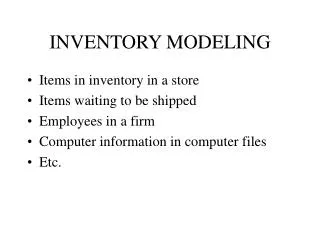
INVENTORY MODELING • Items in inventory in a store • Items waiting to be shipped • Employees in a firm • Computer information in computer files • Etc.
COMPONENTS OF AN INVENTORY POLICY • Q = the amount to order (the order quantity) • R = when to reorder (the reorder point)
BASIC CONCEPT • Balance the cost of having goods in inventory to other costs such as: • Order Cost • Purchase Costs • Shortage Costs
HOLDING COSTS • Costs of keeping goods in inventory • Cost of capital • Rent • Utilities • Insurance • Labor • Taxes • Shrinkage, Spoilage, Obsolescence
Holding Cost RateAnnual Holding Cost Per Unit • These factors, individually are hard to determine • Management (typically the CFO) assigns a holding cost rate, H, which is a percentage of the value of the item, C • Annual Holding Cost Per Unit, Ch Ch = HC (in $/item in inv./year)
PROCUREMENT COSTS • When purchasing items, this cost is known as the order cost, CO (in $/order) • These are costs associated with the ordering process that are independent of the size of the order-- invoice writing or checking, phone calls, etc. • Labor • Communication • Some transportation
PROCUREMENT COSTS • When these costs are associated with producing items for sale they are called set-up costs (still labeled CO-- in $/setup) • Costs associated with getting the process ready for production (regardless of the production quantity) • Readying machines • Calling in, shifting workers • Paperwork, communications involved
PURCHASE/PRODUCTION COSTS • These are the per unit purchase costs, C, if we are ordering the items from a supplier • These are the per unit production costs, C, if we are producing the items for sale
CUSTOMER SATISFACTION COSTS • Shortage/Goodwill Costs associated with being out of stock • goodwill • loss of future sales • labor/communication • Fixed administrative costs = ($/occurrence) • Annualized Customer Waiting Costs = Cs ($/item short/year)
BASIC INVENTORY EQUATION (Total Annual Inventory Costs) = (Total Annual Order/Setup-Up Costs) + (Total Annual Holding Costs) + (Total Annual Purchase/Production Costs) + (Total Annual Shortage/Goodwill Costs) • This is a quantity we wish to minimize!!
REVIEW SYSTEMS • Continuous Review -- • Items are monitored continuously • When inventory reaches some critical level, R, an order is placed for additional items • Periodic Review -- • Ordering is done periodically (every day, week, 2 weeks, etc.) • Inventory is checked just prior to ordering to determine an order quantity
TIME HORIZONS • Infinite Time Horizon • Assumes the process has and will continue “forever” • Single Period Models • Ordering for a one-time occurence
EOQ-TYPE MODELS • EOQ (Economic Order Quantity-type models assume: • Infinite Time Horizon • Continuous Review • Demand is relatively constant
THE BASIC EOQ MODEL • Order the same amount, Q, each time • Reordering is instantaneous • Demand is relatively constant at D items/yr. • Infinite Time Horizon/Continuous Review • No shortages • Since reordering is instantaneous
Receive order Inventory depletion (demand rate) Q Q — 2 On-hand inventory (units) Average cycle inventory 1 cycle Time Economic Order Quantity Figure 13.2
THE EOQ COST COMPONENTS • Total Annual Order Costs: • (Cost/order)(average # orders per year) = CO(D/Q) • Total Annual Holding Costs: • (Cost Per Item in inv./yr.)(Average inv.) = Ch(Q/2) • Total Annual Purchase Costs: • (Cost Per Item)(Average # items ordered/yr.) = CD
Total cost = Holding Cost + Set-up Cost Annual cost (dollars) Holding cost Ordering cost Lot Size (Q) Economic Order Quantity Figure 13.3
THE EOQ TOTAL COST EQUATION • TC(Q) = CO(D/Q) + Ch(Q/2) + CD • This a function in one unknown (Q) that we wish to minimize
SOLVING FOR Q* • TC(Q) = CO(D/Q) + Ch(Q/2) + CD
THE REORDER POINT, r* • Since reordering is instantaneous, r* = 0 • MODIFICATION -- fixed lead time = L yrs. r* = LD But demand was only approximately constant so we may wish to carry some safety stock (SS) to lessen the likelihood of running out of stock • Then, r* = LD + SS
TOTAL ANNUAL COST • The optimal policy is to order Q* when supply reaches r* • TC(Q*) = COD/Q* + (Ch/2)(Q*) + CD + ChSS <==variable cost==> fixed safety cost stock cost • The optimal policy minimizes the total variable cost, hence the total annual cost
TOTAL VARIABLE COST CURVE • Ignoring fixed costs and safety stock costs:
EXAMPLE -- ALLEN APPLIANCE COMPANY • Juicer Sales For Past 10 weeks 1. 105 6. 120 2. 115 7. 135 3. 125 8. 115 4. 120 9. 110 5. 125 10. 130 • Using 10-period moving average method, D = (105 + 115 + …+ 130)/10 = 120/ wk = 6240/yr
ALLEN APPLIANCE COSTS • Juicers cost $10 each and sell for $11.85 • Cost of money = 10% • Other misc. costs associated with inventory = 4% • Labor, postage, telephone charges/order = $8 • Workers paid $12/hr. -- 20 min. to unload an order H = .10 + .04 = .14; Ch = .14(10) = $1.40 CO = $8 + (1/3 hr.)*($12/hr.) = $8 + $4 = $12
OPTIMAL QUANTITIES • Total Order Cost = COD/Q* = (12)(6240)/327 = $228.99 • Total Holding Cost = (Ch/2)Q* = (1.40/2)(327) =$228.90 • (Total Order Cost = Total Holding Cost -- except for roundoff) • # Orders Per Year = D/Q* = 6240/327 = 19.08 • Time between orders (Cycle Time) = Q*/D = 327/6240 = .0524 years = 2.72 weeks
TOTAL ANNUAL COST • Total Variable Cost = Total Order Cost + Total Holding Cost = $228.99 + $228.90 = $457.89 • Total Fixed Cost = CD = 10(6240) = $62,400 • Total Annual Cost = $457.89 + $62,400 = $62,857.89
WHY IS EOQ MODEL IMPORTANT? • No real-life model really is an EOQ model • Many models are variants of EOQ-type models • Many situations can be approximated by EOQ models • The EOQ model is relatively insensitive to some pretty major errors in input parameters
INSENSIVITY IN EOQ MODELS • We cannot affect fixed costs, only variable costs TV(Q) = COD/Q + (Ch/2)(Q) Now, suppose D really = 7500 (>20% error) • We did not know this and got Q* = 327 TV(327) = ((12)(7500))/327 + (1.40/2)(327) =$504.13 Q* should have been: SQRT(2(12)(7500)/1.40) = 359 TV(359) = ((12)(7500))/359 + (1.40/2)(359) =$502.00 • This is only a 0.4% increase in the TVCost
DETERMINING A REORDER POINT, r* (Without Safety Stock) • Suppose lead time is 8 working days • The company operates 260 days per year • r* = LD where L and D are in the same time units • L = 8/260 .0308 yrs D = 6240 /year r* = .0308(6240) 192 OR, L = 8 days; D/day = 6240/260 = 24 r* = 8(24) = 192
ACTUAL DEMAND DISTRIBUTION • Suppose we can assume that demand follows a normal distribution • This can be checked by a “goodness of fit” test • From our data, over the course of a week, W, we can approximate W by (105 + … + 130) = 120 • W2 sW2 = ((1052 +…+1302) - 10(120)2)/9 83.33
DEMAND DISTRIBUTION DURING 8 -DAY LEAD TIME • Normal • 8 days = 8/5 = 1.6 weeks, so • L = (1.6)(120) = 192 • L2 (1.6)(83.33) = 133.33 • L
SAFETY STOCK • Suppose we wish a cycle service level of 99% • WE wish NOT to run out of stock in 99% of our inventory cycles • Reorder point, r* = L + z.01 L= 192 + 2.33(11.55) 219 • 219 - 192 = 27 units = safety stock = 2.33(11.55) • Safety stock cost = ChSS = 1.40(27) = $37.80 • This should be added to the TOTAL ANNUAL COST
OTHER EOQ-TYPE MODELS • Quantity Discount Models • Production Lot Size Models • Planned Shortage Model ALL SEEK TO MINIMIZE THE TOTAL ANNUAL COST EQUATION
QUANTITY DISCOUNTS • All-units vs. incremental discounts ALL UNITS DISCOUNTS FOR ALLEN Quantity Unit Cost < 300 $10.00 300-600 $ 9.75 600-1000 $ 9.50 1000-5000 $ 9.40 5000 $ 9.00
PIECEWISE APPROACH • For each piece of the total cost equation, the minimum cost for the piece is at an end point or at its Q* • If Q* for a piece lies: • above the upper interval limit -- ignore this piece • within this piece -- it is optimal for this piece • below the lower interval limit -- the lower interval limit is optimal for this piece • Calculate the total annual cost using the best value for Q for each piece, and choose the lowest
QUANTITY DISCOUNT APPROACH FOR ALLEN • When C changes, only Ch changes in the formula for Q* since Ch = .14C Quantity Unit Cost Ch Q* Best Q TC < 300 $10.00 $1.40 327 ---- ---- 300-600 $ 9.75 $1.365 331 331 $61,292 600-1000 $ 9.50 $1.33 336 600 $59,804 1000-5000 $ 9.40 $1.316 337 1000 $59,389 5000 $ 9.00 $1.26 345 5000 $59,325 • ORDER 5000
OTHER CONSIDERATIONS • 5000 is 5000/6240 = .8 years = 9.6 months supply • May not wish to order that amount • Company policy may be: DO NOT ORDER MORE THAN A 3-MONTHS SUPPLY = 6240/4 = 1560 • If that is the case, since 1560 is in the interval from 1000 - 5000 and the best Q in that interval is 1000, 1000 should be ordered
PRODUCTION LOT SIZE PROBLEMS • We are producing at a rate P/yr. That is greater than the demand rate of D/yr. • Inventory does not “jump” to Q but builds up to a value IMAX that is reached when production is ceased • Length of a production time = Q/P • IMAX = P(Q/P) - D(Q/P) = (1-D/P)Q • Average inventory = IMAX/2 = ((1-D/P)/2)Q
Economic Production Quantity On-hand Inventory Time Figure G.1
Economic Production Quantity Production quantity Q On-hand Inventory Time Figure G.1
Economic Production Quantity Production quantity Q Demand during production interval On-hand Inventory p - d Time Figure G.1
Economic Production Quantity Production quantity Q Demand during production interval On-hand Inventory p - d Time Figure G.1
Economic Production Quantity Production quantity Q Demand during production interval On-hand Inventory p - d Time Production and demand Demand only TBO Figure G.1
Economic Production Quantity Production quantity Q Demand during production interval On-hand Inventory p - d Time Production and demand Demand only TBO Figure G.1
Economic Production Quantity Production quantity Q Demand during production interval Imax On-hand Inventory Maximum inventory p - d Time Production and demand Demand only TBO Figure G.1
PRODUCTION LOT SIZE -- TOTAL ANNUAL COST • CO = Set-up cost rather than order cost • Set-up time for production lead time • Q = The production lot size • TC(Q) = CO(D/Q) + Ch((1-D/P)/2)Q + CD
OPTIMAL PRODUCTION LOT SIZE, Q* • TC(Q) = CO(D/Q) + Ch((1-D/P)/2)Q + CD
EXAMPLE-- Farah Cosmetics • Production Capacity 1000 tubes/hr. • Daily Demand 1680 tubes • Production cost $0.50/tube (C = 0.50) • Set-up cost $150 per set-up (CO = 150) • Holding Cost rate: 40% (Ch = .4(.50) = .20) • D = 1680(365) = 613,200 • P = 1000(24)(365) = 8,760,000