Download
1 / 44
510 likes | 853 Vues
Physics and Physical Measurement. Topic 1.2 Measurement and Uncertainties. The S.I. System. Standards of Measurement. SI units are those of the Système International d’Unités adopted in 1960 Used for general measurement in most countries worldwide. Fundamental Quantities.

E N D
Physics and Physical Measurement Topic 1.2 Measurement and Uncertainties
Standards of Measurement • SI units are those of the Système International d’Unités adopted in 1960 • Used for general measurement in most countries worldwide
Fundamental Quantities • Some quantities cannot be measured in a simpler form and for convenience they have been selected as the basic quanitities • They are termed Fundamental Quantities, Units and Symbols
The 7 Fundamentals • Length metre m • Mass kilogram kg • Time second s • Electric current ampere A • Thermodynamic temp Kelvin K • Luminous Intensity candela cd • Amount of a substance mole mol
Derived Quantities • When a quantity involves the measurement of 2 or more fundamental quantities it is called a Derived Quantity • The units of these are called Derived Units
Derived Units Examples… • Acceleration ms-2 • Momentum kgms-1 or Ns Some derived units have been given their own specific names and symbols… • Force N = kg ms-2 • Joule J = kgm2s-2
Standards of Measurement • Scientists and engineers need to make accurate measurements so that they can exchange information • To be useful a standard of measurement must be Invariant, Accessible and Reproducible
3 Standards (FYI – not tested) • The Meter :- the distance traveled by a beam of light in a vacuum over a defined time interval ( 1/299 792 458 seconds) • The Kilogram :- a particular platinum-iridium cylinder kept in Sevres, France • The Second :- the time interval between the vibrations in the caesium atom (1 sec = time for 9 192 631 770 vibrations)
Conversions • You will need to be able to convert from one unit to another for the same quanitity • J to kWh (energy) • J to eV (energy) • Years to seconds (time) • And between other systems and SI ****Note: youshouldbeableto do basicconversionsnow and otherswillbedevelopedthroughouttheyear
SI Format • The accepted SI format is • ms-1 not m/s • ms-2 not m/s/s The IB will recognize work reported with “/”, but will only use the SI format when providing info.
Errors • Errors can be divided into 2 main classes • Random errors • Systematic errors
Mistakes • Mistakes on the part of an individual such as • misreading scales • poor arithmetic and computational skills • wrongly transferring raw data to the final report • using the wrong theory and equations • These are a source of error but are not considered as an experimental error
Systematic Errors • Cause a random set of measurements to be affected in the same way • It is a system or instrument issue
Systematic Errors result from • Badly made instruments • Poorly calibrated instruments • An instrument having a zero error, a form of calibration • Poorly timed actions • Instrument parallax error • Note that systematic errors are not reduced by multiple readings
Random Errors • Are due to unpredictable variations in performance of the instrument and the operator
Random Errors result from • Vibrations and air convection • Misreading • Variation in thickness of surface being measured • Using less sensitive instrument when a more sensitive instrument is available • Human parallax error
Reducing Random Errors • Randomerrors can bereducedbytakingmultiplereadings, and eliminatingobviouslyerroneousresultorbyaveragingtherange of results.
Accuracy • Accuracy is an indication of how close a measurement is to the accepted value indicated by the relative or percentage error in the measurement • An accurate experiment has a low systematic error
Precision • Precision is an indication of the agreement among a number of measurements made in the same way indicated by the absolute error • A precise experiment has a low random error
Reducing the Effects of Random Uncertainties • Take multiple readings • When a series of readings are taken for a measurement, then the arithmetic mean of the reading is taken as the most probable answer • The greatest deviation from the mean is taken as the absolute error
Absolute/fractional errors and percentage errors • We use ± to show an error in a measurement • (208 ± 1) mm is a fairly accurate measurement • (2 ± 1) mm is highly inaccurate
Absolute, fractional, and relative uncertainty Assume we measure something to be 208 ± 1 mm in length... • 1 mm is the absolute uncertainty • 1/208 is the fractional uncertainty (0.0048) • 0.48 % is the relative (percent) uncertainty
Combining uncertainties To determine the uncertainty of a calculated value... • For addition and subtraction, add absolute uncertainities • For multiplication and division add percentage uncertainities • When using exponents, multiply the percentage uncertainty by the exponent
Combining uncertainties • If one uncertainty is much larger than others, the approximate uncertainty in the calculated result may be taken as due to that quantity alone
Significant Figures • Thenumber of significant figures shouldreflecttheprecision of thevaluesused as input data in a calculation Simple rule: • Formultiplication and division, thenumber of significant figures in a resultshouldnotexceedthat of theleast precise valueuponwhichitdepends
Graphical Techniques • Graphing is one of the most valuable tools in data analysis because • it gives a visual display of the relationship between two or more variables • shows which data points do not obey the relationship • gives an indication at which point a relationship ceases to be true • used to determine the constants in an equation relating two variables
You need to be able to give a qualitative physical interpretation of a particular graph
Plotting Graphs • Independent variables are plotted on the x-axis • Dependent variables are plotted on the y-axis • Most graphs occur in the 1st quadrant however some may appear in all 4
Plotting Graphs - Choice of Axis • Experimentally speaking, the dependent variable is plotted on the y axis and the independent variable is plotted on the x axis. • When you are asked to plot a graph of a against b, the first variable mentioned is plotted on the y axis.
Plotting Graphs - Scales • Size of graph should be large, to fill as much space as possible…3/4 rule • choose a convenient scale that is easily subdivided
Plotting Graphs - Labels • Each axis is labeled with the name of the quantity, as well as the relevant unit used… Temperature/K speed/ms-1 • The graph should also be given a descriptive title
Plotting Uncertainties on Graphs • Error bars showing uncertainty are required - short lines drawn from the plotted points parallel to the axes indicating the absolute error of measurement
Plotting Graphs - Line of Best Fit • When choosing the best fit line or curve it is easiest to use a transparent ruler • Position the ruler until it lies along an ideal line • The line or curve does not have to pass through every point • Do not assume that all lines should pass through the origin • Do not do play connect the dots!
y x Uncertainties on a Graph Notice that the best fitting line or curve is one that passes through the error bars of the plotted points. A straight line could not accomplish that with this data set
Analysing the Graph • Often a relationship between variables will first produce a parabola, hyperbole or an exponential growth or decay. These can be transformed to a straight line relationship • General equation for a straight line is y = mx + c • y is the dependent variable, x is the independent variable, m is the gradient and c is the y-intercept
Gradients • Gradient = vertical run / horizontal run gradient = y / x • Don´t forget to give the units of the gradient • In lab work, always report the maximum and minimum gradient
Areas under Graphs • The area under a graph is a useful tool. For example… • on a force vs. displacement graph the area is work (N x m = J) • on a speed time graph the area is distance (ms-1 x s = m) • Again, don´t forget the units of the area
y x Standard Graphs - linear graphs • A straight line passing through the origin shows proportionality y x y = k x k = rise/run Where k is the constant of proportionality
y y x x2 Standard Graphs - parabola • A parabola shows that y is directly proportional to x2 • i.e. y x2 or y = kx2 • where k is the constant of proportionality
y y x 1/x Standard Graphs - hyperbola • A hyperbola shows that y is inversely proportional to x • i.e. y 1/xor y = k/x • where k is the constant of proportionality
y y x 1/x2 Standard Graphs - hyperbola again • An inverse square law graph is also a hyperbola • i.e. y 1/x2 or y = k/x2 • where k is the constant of proportionality