Parallel Computers

1. Chapter 1 Parallel Computers

2. Demand for Computational Speed • Continual demand for greater computational speed from a computer system than is currently possible • Areas requiring great computational speed include numerical modeling and simulation of scientific and engineering problems. • Computations must be completed within a “reasonable” time period.

3. Grand Challenge Problems One that cannot be solved in a reasonable amount of time with today’s computers. Obviously, an execution time of 10 years is always unreasonable. Examples • Modeling large DNA structures • Global weather forecasting • Modeling motion of astronomical bodies.

4. Weather Forecasting • Atmosphere modeled by dividing it into 3-dimensional cells. • Calculations of each cell repeated many times to model passage of time.

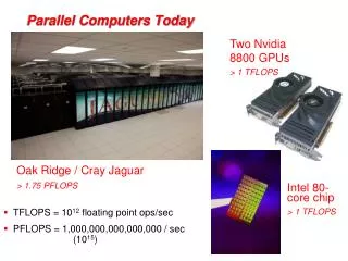
5. Global Weather Forecasting Example • Suppose whole global atmosphere divided into cells of size 1 mile  1 mile  1 mile to a height of 10 miles (10 cells high) - about 5  108 cells. • Suppose each calculation requires 200 floating point operations. In one time step, 1011 floating point operations necessary. • To forecast the weather over 7 days using 1-minute intervals, a computer operating at 1Gflops (109 floating point operations/s) takes 106 seconds or over 10 days. • To perform calculation in 5 minutes requires computer operating at 3.4 Tflops (3.4  1012 floating point operations/sec).

6. Modeling Motion of Astronomical Bodies • Each body attracted to each other body by gravitational forces. Movement of each body predicted by calculating total force on each body. • With N bodies, N - 1 forces to calculate for each body, or approx. N2 calculations. (N log2 N for an efficient approx. algorithm.) • After determining new positions of bodies, calculations repeated.

7. A galaxy might have, say, 1011 stars. • Even if each calculation done in 1 ms (extremely optimistic figure), it takes 109 years for one iteration using N2 algorithm and almost a year for one iteration using an efficient N log2 N approximate algorithm.

8. Astrophysical N-body simulation by Scott Linssen (undergraduate UNC-Charlotte student).

9. Parallel Computing • Using more than one computer, or a computer with more than one processor, to solve a problem. Motives • Usually faster computation - very simple idea - that n computers operating simultaneously can achieve the result n times faster - it will not be n times faster for various reasons. • Other motives include: fault tolerance, larger amount of memory available, ...

10. Background • Parallel computers - computers with more than one processor - and their programming - parallel programming - has been around for more than 40 years.

11. Gill writes in 1958: “... There is therefore nothing new in the idea of parallel programming, but its application to computers. The author cannot believe that there will be any insuperable difficulty in extending it to computers. It is not to be expected that the necessary programming techniques will be worked out overnight. Much experimenting remains to be done. After all, the techniques that are commonly used in programming today were only won at the cost of considerable toil several years ago. In fact the advent of parallel programming may do something to revive the pioneering spirit in programming which seems at the present to be degenerating into a rather dull and routine occupation ...” Gill, S. (1958), “Parallel Programming,” The Computer Journal, vol. 1, April, pp. 2-10.

12. Speedup Factor ts Execution time using one processor (best sequential algorithm) S(p) = where ts is execution time on a single processor and tp is execution time on a multiprocessor. S(p) gives increase in speed by using multiprocessor. Use best sequential algorithm with single processor system. Underlying algorithm for parallel implementation might be (and is usually) different. tp Execution time using a multiprocessor with p processors

13. Speedup factor can also be cast in terms of computational steps: Can also extend time complexity to parallel computations. Number of computational steps using one processor S(p) = Number of parallel computational steps with p processors

14. Maximum Speedup Maximum speedup is usually p with p processors (linear speedup). Possible to get superlinear speedup (greater than p) but usually a specific reason such as: • Extra memory in multiprocessor system • Nondeterministic algorithm

15. Maximum Speedup Amdahl’s law t s ft (1 - f ) t s s Serial section Parallelizable sections (a) One processor (b) Multiple processors p processors (1 - f ) t / p s t p

16. Speedup factor is given by: This equation is known as Amdahl’s law

17. Speedup against number of processors f = 0% 20 16 12 f = 5% 8 f = 10% f = 20% 4 4 8 12 16 20 Number of processors , p

18. Even with infinite number of processors, maximum speedup limited to 1/f. Example With only 5% of computation being serial, maximum speedup is 20, irrespective of number of processors.

19. Superlinear Speedup example - Searching (a) Searching each sub-space sequentially Start Time t s t /p s Sub-space D t search x t /p s Solution found x indeterminate

20. (b) Searching each sub-space in parallel D t Solution found

21. Speed-up then given by t s ´ D x + t p S(p) = D t

22. Worst case for sequential search when solution found in last sub-space search. Then parallel version offers greatest benefit, i.e. p – 1 ´ D t + t s p ® ¥ S(p) = D t D as t tends to zero

23. Least advantage for parallel version when solution found in first sub-space search of the sequential search, i.e. Actual speed-up depends upon which subspace holds solution but could be extremely large. D t S(p) = = 1 D t

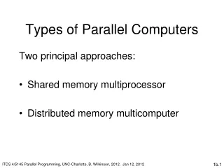
24. Types of Parallel Computers Two principal types: • Shared memory multiprocessor • Distributed memory multicomputer

25. Shared Memory Multiprocessor

26. Conventional Computer Consists of a processor executing a program stored in a (main) memory: Each main memory location located by its address. Addresses start at 0 and extend to 2b - 1 when there are b bits (binary digits) in address. Main memory Instr uctions (to processor) Data (to or from processor) Processor

27. Shared Memory Multiprocessor System Natural way to extend single processor model - have multiple processors connected to multiple memory modules, such that each processor can access any memory module : Memory module One address space Interconnection network Processors

28. Simplistic view of a small shared memory multiprocessor Examples: • Dual Pentiums • Quad Pentiums Processors Shared memory Bus

29. Quad Pentium Shared Memory Multiprocessor Processor Processor Processor Processor L1 cache L1 cache L1 cache L1 cache L2 Cache L2 Cache L2 Cache L2 Cache Bus interface Bus interface Bus interface Bus interface Processor/ memory b us I/O interf ace Memory controller I/O b us Memory Shared memory

30. Programming Shared Memory Multiprocessors • Threads - programmer decomposes program into individual parallel sequences, (threads), each being able to access variables declared outside threads. Example Pthreads • Sequential programming language with preprocessor compiler directives to declare shared variables and specify parallelism. Example OpenMP - industry standard - needs OpenMP compiler

31. Sequential programming language with added syntax to declare shared variables and specify parallelism. Example UPC (Unified Parallel C) - needs a UPC compiler. • Parallel programming language with syntax to express parallelism - compiler creates executable code for each processor (not now common) • Sequential programming language and ask parallelizing compiler to convert it into parallel executable code. - also not now common

32. Message-Passing Multicomputer Complete computers connected through an interconnection network: Interconnection network Messages Processor Local memory Computers

33. Interconnection Networks • Limited and exhaustive interconnections • 2- and 3-dimensional meshes • Hypercube (not now common) • Using Switches: • Crossbar • Trees • Multistage interconnection networks

34. Two-dimensional array (mesh) Computer/ Links processor Also three-dimensional - used in some large high performance systems.

35. Three-dimensional hypercube

36. Four-dimensional hypercube Hypercubes popular in 1980’s - not now

37. Crossbar switch Memor ies Switches Processors

38. Tree Root Switch Links element Processors

39. Multistage Interconnection NetworkExample: Omega network 2 ´ 2 switch elements (straight-through or crossover connections) 000 000 001 001 010 010 011 011 Inputs Outputs 100 100 101 101 110 110 111 111

40. Distributed Shared Memory Making main memory of group of interconnected computers look as though a single memory with single address space. Then can use shared memory programming techniques. Interconnection netw or k Messages Processor Shared memory Computers

41. Flynn’s Classifications Flynn (1966) created a classification for computers based upon instruction streams and data streams: • Single instruction stream-single data stream (SISD) computer Single processor computer - single stream of instructions generated from program. Instructions operate upon a single stream of data items.

42. Multiple Instruction Stream-Multiple Data Stream (MIMD) Computer General-purpose multiprocessor system - each processor has a separate program and one instruction stream is generated from each program for each processor. Each instruction operates upon different data. Both the shared memory and the message-passing multiprocessors so far described are in the MIMD classification.

43. Single Instruction Stream-Multiple Data Stream (SIMD) Computer • A specially designed computer - a single instruction stream from a single program, but multiple data streams exist. Instructions from program broadcast to more than one processor. Each processor executes same instruction in synchronism, but using different data. • Developed because a number of important applications that mostly operate upon arrays of data.

44. Multiple Program Multiple Data (MPMD) Structure Within the MIMD classification, each processor will have its own program to execute: Program Program Instructions Instructions Processor Processor Data Data

45. Single Program Multiple Data (SPMD) Structure Single source program written and each processor executes its personal copy of this program, although independently and not in synchronism. Source program can be constructed so that parts of the program are executed by certain computers and not others depending upon the identity of the computer.

46. Networked Computers as a Computing Platform • A network of computers became a very attractive alternative to expensive supercomputers and parallel computer systems for high-performance computing in early 1990’s. • Several early projects. Notable: • Berkeley NOW (network of workstations) project. • NASA Beowulf project.

47. Key advantages: • Very high performance workstations and PCs readily available at low cost. • The latest processors can easily be incorporated into the system as they become available. • Existing software can be used or modified.

48. Software Tools for Clusters • Based upon Message Passing Parallel Programming: • Parallel Virtual Machine (PVM) - developed in late 1980’s. Became very popular. • Message-Passing Interface (MPI) - standard defined in 1990s. • Both provide a set of user-level libraries for message passing. Use with regular programming languages (C, C++, ...).

49. Beowulf Clusters* • A group of interconnected “commodity” computers achieving high performance with low cost. • Typically using commodity interconnects - high speed Ethernet, and Linux OS. * Beowulf comes from name given by NASA Goddard Space Flight Center cluster project.

50. Cluster Interconnects • Originally fast Ethernet on low cost clusters • Gigabit Ethernet - easy upgrade path More Specialized/Higher Performance • Myrinet - 2.4 Gbits/sec - disadvantage: single vendor • cLan • SCI (Scalable Coherent Interface) • QNet • Infiniband - may be important as infininband interfaces may be integrated on next generation PCs