Group Analysis: 2 nd level
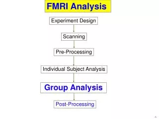
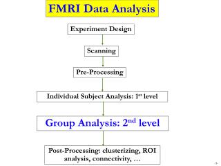
FMRI Data Analysis. Experiment Design. Scanning. Pre-Processing. Individual Subject Analysis: 1 st level. Group Analysis: 2 nd level. Post-Processing: clusterizing, ROI analysis, connectivity, …. Overview Why do we need to do group analysis? Fixed-effects analysis

Group Analysis: 2 nd level
E N D
Presentation Transcript
FMRI Data Analysis Experiment Design Scanning Pre-Processing Individual Subject Analysis: 1st level Group Analysis: 2nd level Post-Processing: clusterizing, ROI analysis, connectivity, …
Overview • Why do we need to do group analysis? • Fixed-effects analysis • Mixed-effects analysis • Nonparametric approach • 3dWilcoxon,3dMannWhitney, 3dKruskalWallis, 3dFriedman • Parametric approach • Traditional parametric analysis • Use effect size only: linear combination of regression coefficients () • 3dttest, 3dANOVA/2/3, 3dRegAna, GroupAna, 3dLME • New group analysis method • Both effect sizeand precision: mixed-effects meta analysis (MEMA) • 3dMEMA
Group Analysis: Fixed-Effects Analysis • Number of subjects n < 6 • Case study: difficult to generalize to whole population • Simple approach (3dcalc) • t = ∑tii/√n • Sophisticated approach • Fixed-effects meta analysis (3dcalc): weighted least squares • β = ∑wiβi/∑wi • t = β∑wi/√n, wi = ti/βi = weight for ith subject • Direct fixed-effects analysis (3dDeconvolve/3dREMLfit) • Combine data from all subjects and then run regression
Group Analysis: Mixed-Effects Analysis • Non-parametric approach • 4 < number of subjects < 10 • No assumption of data distribution (e.g., normality) • statistics based on ranking • Individual and group analyses: separate • Parametric approach • Number of subjects > 10 • Random effects of subjects: usually Gaussian distribution • Individual and group analyses: separate
Mixed-Effects: Non-Parametric Analysis • Programs: roughly equivalent to permutation tests • 3dWilcoxon (~ paired t-test) • 3dMannWhitney(~ two-sample t-test) • 3dKruskalWallis(~ between-subjects with 3dANOVA) • 3dFriedman(~one-way within-subject with 3dANOVA2) • Pros: Less sensitive to outliers (more robust) • Cons • Multiple testing correction limited with FDR (3dFDR) • Less flexible than parametric tests • Can’t handle complicated designs with more than one fixed factor • Can’t handle covariates
Mixed-Effects: Basic concepts in parametric approach • Fixed factor/effect • Treated as a fixed variable (constant) in the model • Categorization of experiment conditions (modality: visual/audial) • Group of subjects (gender, normal/patients) • All levels of the factor are of interest • Fixed in the sense statistical inferences • apply only to the specific levels of the factor • don’t extend to other potential levels that might have been included • Random factor/effect • Treated as a random variable in the model: exclusively subject in FMRI • average + effects uniquely attributable to each subject: e.g. N(μ, σ2) • Each individual subject is of NO interest • Random in the sense • subjects serve as a random sample (representation) from a population • inferences can be generalized to a hypothetical population
Mixed-Effects: Mixed-Effects Analysis • Programs • 3dttest(one-sample, two-sample and paired t) • 3dANOVA (one-way between-subject) • 3dANOVA2 (one-way within-subject, 2-way between-subjects) • 3dANOVA3 (2-way within-subject and mixed, 3-way between-subjects) • 3dRegAna(regression/correlation, plus covariates) • GroupAna(Matlab package for up to 5-way ANOVA) • 3dLME(R package for all sorts of group analysis) • 3dMEMA(R package for meta analysis, t-tests plus covariates)
Mixed-Effects: Which program should I use? • Two perspectives: batch vs. piecemeal • Experiment design • Factors/levels, balancedness • * ANOVA: main effects, interactions, simple effects, contrasts, … • * Linear mixed-effects model • Most people are educated in this traditional paradigm! • Pros: get everything you want in one batch model • Cons: F-stat for main effect and interaction is difficult to comprehend sometimes: a condensed/summarized test with vague information when levels/factors greater than 2 (I don’t like F-test personally!!! Sorry, Ronald A. Fisher…) • Tests of interest • Simple and straightforward: Focus on each individual test, attack one at a time! • Mainly t-stat: one-sample, paired, two-sample • All main effects and interactions can be broken into multiple t-tests
Jack of All Trades (well, almost): 3dttest • Basic usage • One-samplet • One group: simple effect; Example: 15 subjects under condition A with H0:μA= 0 • Two-samplet • Two groups: Compare one group with another • ~ 1-way between-subject (3dANOVA2 -type 1) • Unequal sample sizes allowed • Homoskedasticity vs. heteroskedasticity: -unpooled • Example: 15 TD subjects vs. 13 autism subjects - H0:μA = μB • Pairedt • Two conditions of one group: Compare one condition with another • ~ one-way within-subject (3dANOVA2 -type 3) • ~ one-sample t on individual contrasts • Example: Difference of visual and auditory conditions for 10 subjects with H0:μV = μA • Output: 2 values (effect and t) • Versatile program: Most tests can be done with 3dttest- piecemeal vs. bundled • -mask option unavailable but desirable!
Model type, • 3dttest: Example • Paired t-test 3dttest -prefix ttest_V-A –paired \ -set1 \ 'OLSQ.FP.betas+tlrc[1]' \ 'OLSQ.FR.betas+tlrc[1]' \ …… 'OLSQ.GM.betas+tlrc[1]' \ -set2 \ 'OLSQ.FP.betas+tlrc[0]' \ 'OLSQ.FR.betas+tlrc[0]' \ …… 'OLSQ.GM.betas+tlrc[0]' Input files for Arel condition Input files for Vrel condition
ANOVA program 1: 3dANOVA • Generalization of two-sample t-test • One-way between-subject: 2 or more groups of subjects • H0: no difference across all levels (groups) • Examples of groups: gender, age, genotype, disease, etc. • Unequal sample sizes allowed • Assumptions • Normally distributed with equal variance across groups • Results: 2 values (% and t) • 3dANOVA vs. 3dttest • Equivalent with 2 levels (groups) if equal variance is assumed • More than 2 levels (groups): Can run multiple two-sample t-test • 3dttest allows heteroscedasticity (unequal variance across groups)
ANOVA program 2: 3dANOVA2 • Designs • One-way within-subject (type 3) • Major usage • Compare conditions in one group • Extension and equivalence of paired t • Two-way between-subjects (type 1) • 1 condition, 2 classifications of subjects • Extension and equivalence two-sample t • Unbalanced designs disallowed: Equal number of subjects across groups • Output • Main effect (-fa): F • Interaction for two-way between-subjects (-fab): F • Contrast testing • Simple effect (-amean) • 1st level (-acontr, -adiff): among factor levels • 2nd level (interaction) for two-way between-subjects • 2 values per contrast: % and t
Model type, Factor levels • 3dANOVA2: Example • Two factors: A – condition (fixed, 2 levels); B – subject (random, 10 levels). • Script s1.3dANOVA2 under ~/AFNI_data6/group_results/ 3dANOVA2 -type 3 -alevels 2 -blevels 10 \ -mask mask+tlrc \ -dset 1 1 'OLSQ.FP.betas+tlrc[Vrel#0_Coef]’ \ -dset 2 1 'OLSQ.FP.betas+tlrc[Arel#0_Coef]’ \ -dset 1 2 'OLSQ.FR.betas+tlrc[Vrel#0_Coef]’ \ -dset 2 2 'OLSQ.FR.betas+tlrc[Arel#0_Coef]’ \ …… -dset 1 10 'OLSQ.GM.betas+tlrc[Vrel#0_Coef]' \ -dset 2 10 'OLSQ.GM.betas+tlrc[Arel#0_Coef]' \ -amean 1 V \ -amean 2 A \ -adiff 1 2 VvsA \ -fa FullEffect \ -bucket anova.VA Input for each cell in ANOVA table: Totally 2X10 = 20 t tests: one-sample type t test: two-paired F test: main effect Output: bundled All the F/t-tests here can be obtained with 3dttest!
ANOVA program 3:3dANOVA3 • Designs • Two-way within-subject (type 4): Crossed design AXBXC • Generalization of paired t-test • One group of subjects • Two categorizations of conditions: A and B • Two-way mixed (type 5): Nested design BXC(A) • Two or more groups of subjects (Factor A): subject classification, e.g., gender • One category of condition (Factor B) • Nesting: balanced • Three-way between-subjects (type 1) • 3 categorizations of groups • Output • Main effect (-fa and -fb) and interaction (-fab): F • Contrast testing • 1st level: -amean, -adiff, -acontr, -bmean, -bdiff, -bcontr • 2nd level: -abmean, -aBdiff, -aBcontr, -Abdiff, -Abcontr • 2 values per contrast : % and t
ANOVA program 4: GroupAna • Pros • Matlab script package for up to 5-way ANOVA • Can handle both volume and surface data • Can handle following unbalanced designs (two-sample t type): • 3-way ANOVA type 3: BXC(A) • 4-way ANOVA type 3: BXCXD(A) • 4-way ANOVA type 4: CXD(AXB) • Cons • Use a commercial packag: requires Matlab plus Statistics Toolbox • Difficult to test and interpret simple effects/contrasts • Complicated design, and compromised power • GLM approach (slow): heavy duty computation: minutes to hours • Input with lower resolution recommended • Resample with adwarp -dxyz # and 3dresample • See http://afni.nimh.nih.gov/sscc/gangc for more info
Linear Mixed-Effects Analysis: 3dLME • Pros • R package: open source platform • Linear mixed-effects (LME) modeling • Versatile: handles almost all situations in one package • Unbalanced designs (unequal number of subjects, missing data, etc.) • ANOVA and ANCOVA, but unlimited factors and covariates • Able to handle HRF modeling with basis functions • Violation of sphericity: heteroscedasticity, variance-covariance structure • Model fine-tuning • Cons • High computation cost (lots of repetitive calculation) • Controversial regarding degrees of freedom • See http://afni.nimh.nih.gov/sscc/gangc/lme.html for more information
Linear Mixed-Effects Analysis: 3dLME • Running LME: HRF modeled with 6 tents • Null hypothesis: no HRF difference between two conditions Data:Volume <-- either Volume or Surface Output:test <-- any string (no suffix needed) MASK:Mask+tlrc.BRIK <-- mask dataset FixEff:Time-1 <-- model formula for fixed effects COV: <-- covariate list RanEff: 1 <-- random effect specification VarStr:weights=varIdent(form=~1|Time) <-- heteroscedasticity? CorStr:correlation=corAR1(form=~Order|Subj) <-- correlation structure SS:sequential <-- sequential or marginal Clusters:4 Subj Time TimeOrder InputFile Jim t1 1 contrastT1+tlrc.BRIK Jim t2 2 contrastT2+tlrc.BRIK ...... Jim t6 6 contrastT6+tlrc.BRIK
Mixed-Effects Meta Analysis:3dMEMA • Requirements • R installment, plus ‘snow’ package for parallel computing • 3 running modes • Scripting: type ‘3dMEMA –help’ at terminal to see usage • Sequential/interactive mode inside R: source(“~/abin/3dMEMA.R”) • Batch (if answers known): R CMD BATCH Cmds.R myDiary & • Pros • Makes more sense: better statistical properties • Likely more statistically powerful • Less prone to outliers • Provides more diagnostic measures • Can include covariates in the analysis • Cons • Longer runtime • Can’t handle sophisticated situations: basis functions, ANOVAs, …
3dMEMA: example-scripting Paired test: visual-reliable vs. auditory-reliable (script s4.3dMEMA.V-A under AFNI_data6/group_results/ 3dMEMA -prefix mema_V-A -mask mask+tlrc -jobs 4 -max_zeros 3 \ -conditions Vrel Arel –Hktest -model_outliers \ -set Arel \ FP 'REML.FP.bt+tlrc[2]' 'REML.FP.bt+tlrc[3]' \ FR 'REML.FR.bt+tlrc[2]' 'REML.FR.bt+tlrc[3]' \ …… GK 'REML.GK.bt+tlrc[2]' 'REML.GK.bt+tlrc[3]' \ GM 'REML.GM.bt+tlrc[2]' 'REML.GM.bt+tlrc[3]' \ -set Vrel \ FP 'REML.FP.bt+tlrc[0]' 'REML.FP.bt+tlrc[1]’ \ FR 'REML.FR.bt+tlrc[0]' 'REML.FR.bt+tlrc[1]’ \ …… GK 'REML.GK.bt+tlrc[0]' 'REML.GK.bt+tlrc[1]' \ GM 'REML.GM.bt+tlrc[0]' 'REML.GM.bt+tlrc[1]'
3dMEMA: example-interactive/batch • One-sample test: visual-reliable • Sequential/interactive mode on R prompt • Demo here • Batch mode: R CMD BATCH scriptCMD.R myDiary.txt & • Remote running: nohup R CMD BATCH scriptCMD.R myDiary.txt &
3dMEMA: comparison with 3dttest • Majority of significant voxels with 3dMEMA gained power with a threshold of 2.0 for t(30)
3dMEMA: comparison with 3dttest • Majority of significant voxels with 3dMEMA gained power (red: 3dMEMA higher; blue: 3dttest higher) with a threshold of 2.0 for t(9).
Why new group analysis approach? • Our ultimate goal is not just to gain statistical power • Old group analysis approach • Take ’sfrom each subject, and run t-test, AN(C)OVA, LME • Three assumptions • Within/intra-subject variability (standard error, sampling error) is relatively small compared to cross/between/inter-subjects variability • Within/intra-subject variability roughly the same across subjects • Normal distribution for cross-subject variability (no outliers) • Violations seem everywhere: violating either can lead to suboptimal/invalid analysis • Common to see 40% up to 100% variability due to within-subject variability • Non-uniform within/intra-subject variability across subjects
How can we do it differently? • For each effect estimate ( or linear combination of ’s) • Information regarding our confidence about the effect? • Reliability/precision/efficiency/certainty/confidence: standard error (SE)! • Smaller SE higher reliability/precision/efficiency/certainty/confidence • SE of an effect = estimated standard deviation (SD) of the effect • t-statistic of the effect • Signal-to-noise or effect vs. uncertainty: t = /SE • SE contained in t-statistic: SE = /t • Trust those ’s with high reliability/precision (small SE) through weighting/compromise • estimate with high precision (lower SE) has more say in the final result • estimate with highuncertainty gets downgraded
Differentiate effects based on precision • Dealing with outliers • Unreliable estimate (small t): small/big + big SE • Will automatically be downgraded • May still slightly bias cross-subjects variability estimate to some extent, leading to unfavorable significance testing, but much better than conventional approach • Reliable estimate (big t): small/big + small SE • Weighting only helps to some extent: if one subject has extremely small SE (big t), the group effect may be dominated by this subject • Needs delicate solutions: fundamentally why outliers? • Brain level: Considering ovariate(s)? Grouping subjects? • Singular voxels: special modeling on cross-subject variance
Running 3dMEMA • Currently available analysis types (+ covariates allowed) • One-sample: one condition with one group • Two-sample: one condition across 2 groups with homoskedasticity (same variability) • Paired-sample: two conditions with one group • Two-sample: one condition across 2 groups with heteroskedasticity (different variability) • Output • Group level: % signal change + Z/t-statistic, τ2 + Q • Individual level: λ + Z for each subject • Modes • Scripting • Sequential mode on terminal • Batch mode: R CMD BATCH cmds.R diary.txt &
3dMEMA limitations • Basis functions? • Stick with 3dLME for now • ANOVA? • Extension difficult • t-tests should be no problem • F-tests? • Some of them boil down to t-tests, for example: F-test for interaction between A and B (both with 2 levels) with “3dANOVA3 -type 5…”: equivalent to t-test for (A1B1-A1B2)-(A2B1-A2B2) or (A1B1-A2B1)-(A1B2-A2B2), but we can say more with t than F: a positive t shows A1B1-A1B2 > A2B1-A2B2 and A1B1-A2B1 > A1B2-A2B2 • Do something for other F in the future?
Covariates • Covariates • May or may not be of direct interest • Confounding, nuisance, or interacting variables • Subject-level (vs. trial-level: handled via amplitude modulation) • Controlling for variability in the covariate • Continuous or discrete? • One-sample model yi = α0+α1xi+δi + i, for ith subject • Two-sample model yi = α0+α1x1i+α2x2i+α3x3i+δi + i • Examples • Age, IQ, brain volume, cortex thickness • Behavioral data
Handling covariates: one group • Centering: tricky business (using age as an example) • yi = α0+α1xi+δi + , for ith subject • Interested in group effect α0 (x=0) while controlling (partialling out) x • α1 - slope (change rate): % signal change per unit of x • Interpretability: group effect α0 at what value of x: mean or any other value?
Covariates: trickier with 2 groups • Center and slope • yi = α0+α1x1i+α2x2i+α3x3i+δi + , for ith subject • x1: group indicator • x2: covariate • x3: group effect in slope (interaction btw group and covariate) • What we’re interested • Group effects α0 and α1 while controlling covariate • Interpretability • Center • Group effect α0 and α1 at what covariate value? • Same or different center across groups? • Slope • same (α3=0) or different (α3≠0) slope across groups
Covariates: scenarios with 2 groups • Center and slope (again using age as an example) • yi = α0+α1x1i+α2x2i+α3x3i+δi + i, for ith subject • Interpretability • Same center and slope (α3=0) • Different center with same slope (α3=0) • Same center with different slope (α3≠0) • Different center and slope (α3≠0)
Start simple: one-sample test • Random-effects: yi=θi+i=α0+δi+i, for ith subject • yi : or linear combination (contrast) of ’s from ith subject • θi=α0+δi: “true” individual effect from ith subject • α0: group effect we’d like to find out • δi : deviation of ith subject from group effect α0, N(0, τ2) • i: sample error from ith subject, N(0, σi2), σi2known! • Special cases • σi2=0 reduced to conventional group analysis: One-sample t: yi = α0 +δi • δi=0 (τ2=0) assumed in fixed-effects (FE) model: Ideally we could find out all possible explanatory variables so only an FE model is necessary! • Mature meta analysis tools for this simple model • Broadly used in clinical trials/epidemiology in recent 20 yrs • A special case of linear mixed-effects model
MEMA with one-sample test • Random-effects: yi = α0 +δi + i, for ith subject • δi ~ N(0, τ2), i ~N(0, σi2), σi2 known, τ2unknown • What can we achieve? • Null hypothesis about group effect H0: α0 = 0 • Checking group heterogeneity H0: τ2= 0 • Any outliers among the subjects? Adding some confounding variable(s)? Grouping subjects? • We know σi2, and pretend we also knew τ2, weighted least squares (WLS) gives • The “best” estimate • BLUE: unbiased with minimum variance • Wake up: Unfortunately we don’t know τ2!!!
Solving MEMA in one-sample case • Estimating τ2: a few approaches • Method of moment (MoM) - DSL • Maximum likelihood (ML) • Restricted/residual/reduced/marginal ML (REML): 3dMEMA • Statistical testing • Group effect α0=0: • Wald or Z-test: assume enough subjects with normal distributions • Go with t-test when in doubt • Heterogeneity test τ2=0: • Outlier identification for each subject through Z-statistic
We don’t limit ourselves to simple case • yi = α0 +α1xi1 +…+αipxip+δi + i, for ith subject • Mixed-effects model or meta regression • yi: or linear combination (contrast) of ’s from ith subject • α0: common group effect we’d like to find out • xij: an indicator/dummy variable showing, for example, group to which ith subject belongs, level at which a factor lies, or a continuous variable such as covariate (e.g., age, IQ) (j=1,…,p) • δi : deviation of ith subject from group effect α0, N(0, τ2) • i: sample error from ith subject, N(0, σi2), σi2 known! • Combine subjects into a concise model in matrix form • yn×1 = Xn×pαp×1+n×1+n×1 • y ~ N(Xα, τ2In+V), V = diag(σ1,…, σn) known, τ2 unknown • Estimate α and τ2simultaneously via maximizing REML
Dealing with outliers • Detection • Ideally we wish to account for anything until having no cross-subject variability: τ2 = 0! • 4 quantities to check cross-subject variability • Cross subject variability (heterogeneity) τ2 • Q for H0: τ2 = 0 • Intra-class correlation (ICC): λ = σi2/(σi2+τ2) • Z statistic of i • Modeling: how to handle outliers in the model? • Ignore those subjects with 2 s.d. away from mean? • Arbitrary: OK with data within 1.9 s.d.? • How about when outliers occur at voxel level? • If throwing away outliers at voxel level, varying DFs across brain?
Modeling outliers • Modeling: how to handle outliers in the model? • Typically a Gaussian for subject deviation:δi~N(0, τ2) • With outliers, assume a Laplace (double exponential) distribution • μ: location parameter • b: scale parameter • Mean=median=mode=μ • Variance = 2b2 • Fatter tail but smaller Var • Estimator of μ is sample median, and ML estimator of b
Modeling outliers • Laplace distribution for outlier modeling • No REML form • Go with ML: variance estimate τ2 might be slightly underestimated • Computation cost: higher • Generally higher statistical power
Moral of a story • Story • Strong activation at individual level and in ROI analysis failed to show up at group level • Result with 3dMEMA showed consistency with individual and ROI analysis • Magic power of 3dMEMA? Relatively robust to some (unreliable) outliers • Check brick labels for all input files foreach subj (S1 S2 S3 …) 3dinfo -verb ${subj}_file+tlrc | grep 'sub-brick #0’ end ++ 3dinfo: AFNI version=AFNI_2008_07_18_1710 (Jul 8 2009) [32-bit] -- At sub-brick #0 ’contr_GLT#0_Coef' datum type is float: -0.78438 to 0.867817 -- At sub-brick #0 ’contr_GLT#0_Coef' datum type is float: -0.444093 to 0.501589 …
Suggested preprocessing steps • Input • and t-statistic from each subject • One sub-brick per input file (3dbucket) • Some suggestions • Slice timing correction and volume registration • Aligning/warping to standard space • Avoid troubling step of warping on t-statistic • Smoothing: 3dBlurToFWHM • Scaling • All input files, and more importantly t-statistic, come from 3dREMLfit instead of 3dDeconvolve • No masking applied at individual level so that no data is lost at group level along the edge of (and sometimes inside) the brain
Overview: 3dMEMA • http://afni.nimh.nih.gov/sscc/gangc/MEMA.html • Meta analysis: compromise between Bayesian and frequentist • Backbone: WLS + maximization of REML or ML of Laplace-Gauss • Currently available types • One-, two-, paired-sample test • Covariates allowed: careful with centering and interaction with groups • Output • Group level: group effect (% sigmal change) and statistics (Z/t), cross-subject heterogeneity τ2 and Q (χ2-test) • Individual level: λ + Z for each subject • Generally more powerful/valid than conventional approach • Relatively robust against most outliers • Moderate computation cost with parallel computing: 3-20 minutes • Limitations • Can’t handle sophisticated types: multiple basis functions; F-test types • Computation cost