Methods for Dummies Second level analysis
Methods for Dummies Second level analysis. By Samira Kazan and Bex Bond Expert: Ged Ridgway. Today’s talk. What is second level analysis? Building on our first level analysis – look at a group Explaining fixed and random effects

Methods for Dummies Second level analysis
E N D
Presentation Transcript
Methods for DummiesSecond level analysis By Samira Kazan and Bex Bond Expert: Ged Ridgway
Today’s talk • What is second level analysis? • Building on our first level analysis – look at a group • Explaining fixed and random effects • How do we generalise our findings to the population at large? • Implementing random effects analysis • Hierarchical models vs. summary statistics approach • Implementing second-level analyses in SPM
1st level analysis – single subject For each participant individually: • Spatial preprocessing • accounting for movement in the scanner • fitting individuals’ scans into a standard space • smoothing and so on for statistical power • …
1st level analysis – single subject For each participant individually: • Set up a General Linear Model for each individual voxel • Y=βX + ε • Y is the activity in the voxel – βX is our prediction of this activity, εis the error of our model in its predictions. • X represents the variables we use to predict the data – mainly, we use the design matrix to specify X, so we can change our predictions between different trial types (levels of X), e.g. seeing famous faces and seeing non-famous faces. Thus need to incorporate stimulus onset times. • We estimate β: how much X affects Y – its significance indicates the predictive value of X
1st level analysis – single subject • In the above GLM, we can also incorporate other predictor variables to improve the model: • Movement parameters • we can measure and thus account for this known error – thus increasing our power • Physiological functions, e.g. Haemodynamic Response Function • modelling how neuronal activity may be transformed into a haemodynamic response by neurophysiology may improve our ability to claim that our data based on the BOLD signal represents ‘activity’
1st level analysis – single subject • For each participant, we get a Maximum Intensity Projection for our contrasts tested • We can see where, on average, this individual showed a significant difference in activation. Can overlay this with structural images. • Remember, the voxels are each analysed individually to build up this map. Also beware multiple comparisons inflating α.
2nd level analysis – across subjects • Significant differences in activation between different levels of X are unlikely to be manifest identically in all individuals. We might ask: • Is this contrast in activation seen on average in the population? • Is this contrast in activation different on average between groups? e.g. males vs. females?
2nd level analysis – across subjects • We need to look at which voxels are showing a significant activation difference between levels of X consistently within a group. • To do this, we need to consider: • the average contrast effect across our sample • the variation of this contrast effect • t tests involve mean divided by standard error of mean
2nd level analysis – Fixed effects analysis (FFX) • Each subject repeats trials of each type many times – the variation amongst the responses recorded for each level of the design matrix (X) for a given subject gives us the within-subjects variance,σw2 • If we take the group effect size as the mean of responses across our subjects, and analyse it with respect to σw2, we can infer which voxels on average show a significant difference in activation between levels of X in our sample… • …and ONLY in our specific sample. We cannot infer anything about the wider population unless we also consider between-subjects variation. This is called fixed-effects analysis.
An illustration (from Poldrack, Mumford and Nichol’s ‘Handbook of fMRI analyses’) Random effects
2nd level analysis – Random effects analysis (RFX) • In order to make inferences about the population from which we assume our subjects are randomly sampled from, we must incorporate this assumption into our model. • To do this, we must consider the between-subject variance (σb2), as well as within subject-variance (σw2) – and estimate the likely variance of the population from which our sample is derived. • This is referred to as “random effects analysis”, as we are assuming that our sample is a random set of individuals from the population.
Take home message • In fMRI, between-subject variance is much greater than within-subject variance. We need to consider both aspects of variance to make any inferences about the wider population, rather than just our sample. • As the population variance is much greater than the within-subjects variance, fixed effects analysis ‘overestimates’ the significance of effects – random effects analysis is more conservative, highlighting the greater effects, that may be seen across the population. Fixed effects may be swayed by outliers.
2nd level analysis – Methods for RFX analysis • Hierarchical model • Estimates subject and group stats at once via iterative looping • Ideal method in terms of accuracy… • …but computationally intensive, and not always practical! • (e.g. adding in subjects means the entire estimation process has to start from scratch again) • Can we get a good, quick approximation? A valid one?
2nd level analysis – Methods for RFX analysis • Summary Statistics Approach • This is what SPM uses! • Involves bringing sample means forward from 1st level analysis. Less computationally demanding! • Generally valid; quite robust • valid when the 1st level design is the same for all subjects (e.g. number of trials) • exact same results as a hierarchical model when the within-subject variance is the same for all subjects – so it’s a good approximation when they are roughly the same • validity undermined by extreme outliers
Overview of SPM Statistical parametric map (SPM) Design matrix Image time-series Kernel Realignment Smoothing General linear model Gaussian field theory Statistical inference Normalisation p <0.05 Template Parameter estimates
Fixed vs. Random Effects in fMRI Fixed-effects • Intra-subject variation Inferences specific to the group Random-effects • Inter-subject variation Inferences generalised to the population Courtesy of [1]
Fixed vs. Random Effects in fMRI Fixed-effects • Is not of interest across a population • Used for a case study • Only source of variation is measurement error (Response magnitude is fixed) Random-effects • If I have to take another sample from the population, I would get the same result • Two sources of variation • Measurement error • Response magnitude is random (population mean magnitude is fixed) Courtesy of [1]
Data set from the Human Connectume Project Courtesy of [2]
This defines the search space for the statistical analysis. Image of the variance of the error and is used to produce spmT images. The estimated resels per voxel (not currently used). beta. images of estimated regression coefficients (parameter estimate). Combined to produce con. images.
Subject 1 Subject 2 Subject 3
Fixed-effects Analysis in SPM Subject 1 Subject 2 Subject 3 multi-subject 1st level design each subjects entered as separate sessions create contrast across all subjects c = [ -1 1 -1 1 -1 1 -1 1 -1 1 -1 1 -1 1 -1 1 -1 1 -1 1 -1 1 -1 1] perform one sample t-test
Random-effects in SPM Used for: • Setting up analysis for random effects
Methods for Random-effects Hierarchical model • Estimates subject & group stats at once • Variance of population mean contains contributions from within- & between- subject variance • Iterative looping computationally demanding Summary statistics approach Most commonly used! • 1stlevel design for all subjects must be the SAME • Sample means brought forward to 2nd level • Computationally less demanding • Good approximation, unless subject extreme outlier
SPM 2nd Level: How to Set-Up Directory for the results of the second level analysis
SPM 2nd Level: How to Set-Up Design - several design types • one sample t-test • two sample t-test • paired t-test • multiple regression • one way ANOVA • (+/-within subject) • full factorial
Two sample T test Group 1 mean Contrasts (1 0) mean group 1 (0 1) mean group 2 (1 -1) mean group 1 - mean group 2 (0.5 0.5) mean (group 1, group 2) Group 2 mean
One way between subject ANOVA • Consider a one-way ANOVA with 4 groups and each group having 3 subjects, 12 observations in total • SPM rule • Number of regressors = number of groups
One way ANOVA H0= G1-G2 C=[1 -1 0 0]
One way ANOVA H0= G1=G2=G3=G4=0 c=
Specifies voxels within image which are to be assessed - 3 masks types: • threshold (voxel > threshold used) • implicit (voxels >0 are used) • explicit (image for implicit mask) - covariates & nuisance variables - 1 value per con*.img
SPM 2nd Level: Results • Click RESULTS • Select your 2nd Level SPM
SPM 2nd Level: Results • 2nd level one sample t-test • Select t-contrast • Define new contrast …. • c = +1 (e.g. A>B) • c = -1 (e.g. B>A) • Select desired contrast
SPM 2nd Level: Results • Select options for displaying result: • Mask with other contrast • Title • Threshold (pFWE, pFDRpUNC) • Size of cluster
SPM 2nd Level: Results • Here are your results… • Now you can view: • Table of results [whole brain] • Look at t-value for a voxel of choice • Display results on anatomy [ overlays ] • SPM templates • mean of subjects • Small Volume Correct
Thank youResources: http://www.fil.ion.ucl.ac.uk/spm/course/slides10-vancouver/04_Group_Analysis.pdf HummanConnectome Project (Working Memory example) http://www.humanconnectome.org/documentation/Q1/Q1_Release_Reference_Manual.pdf 3) Previous MFD slides Thanks to Ged Ridgway