Download
1 / 37
370 likes | 492 Vues
Explore different methods for estimating volatility in energy portfolios, with a focus on option pricing and risk management. Learn about historical vs. implied volatility, modeling energy prices, and challenges in supply and demand analysis.

E N D
Volatility Estimation Techniques for Energy Portfolios Vince Kaminski Research Group Houston, January 30, 2001
The market is as much dependent on economists, as weather on meteorologists. George Herbert Wells
Outline • Definition of volatility • Importance of volatility to option pricing and financial analysis • Recent experience of volatility of power prices in the United States • Estimation of volatility from historical data • Volatility derived from a structural model
Importance of Volatility • Critical input to option pricing models • More accurate volatility forecasts increase the efficiency of hedging strategies • Used as a measure of risk in models applied in • Risk management (value-at-risk) • Portfolio selection • Margining
Different Types of Volatility • Volatility - a statistical measure of price return variability • Historical volatility: volatility estimated from historical prices • Implied volatility: volatility calculated from option prices observed in the market place • Volatility implied by a fundamental model
Different Types of Volatility (2) • Different definitions of volatility reflect different modeling philosophies • Reduced form approach • Historical / implied volatility approach is based on the use of a formal statistical model • Reduced from approach assumes that a single, general form equation describes price dynamics • Structural model assumes that the balance of supply and demand in the underlying markets can be modeled • Partial or general equilibrium models
Option Pricing Technology • Prices evolve in a real economy and are characterized by certain empirical probability distributions • Options are priced in a risk-neutral economy: a theoretical concept. Prices are characterized in terms of risk-neutral (i.e. fake) probability distributions. • If the math is done correctly, option prices in both economies will be identical • Volatility constitutes the bridge between the two economies • The risk-neutral economy can be constructed if a replicating (hedging) portfolio can be created
Option Pricing Technology (2) • The only controversial input an option trader has to provide in order to price an option is the volatility • The shortcomings of an option pricing model are addressed by adjusting the volatility assumption • The approach developed for financial options has been applied to energy commodities in a fairly mechanical way • The inadequacy of this framework for energy commodities is becoming painfully obvious
Modeling Energy Prices • Energy prices have split personality (Dragana Pilipovic) • Traditional modeling tools (Geometric Brownian Motion) may apply to long-term forward prices • As we get closer to delivery, the price dynamics changes • Gapping behavior of spot prices and the front of the forward curve • Prices may be negative or equal to zero
Modeling Energy Prices • Traditional answers to modeling problems seem not to perform well • mean reversion • seasonality of the mean level • different rate of mean reversion for positive and negative deviations from the mean • jump-diffusion processes • asymmetric jumps with a positive bias • one can speak rather of a floor-reversion
Limitations of the Arbitrage Argument • In many cases it is impossible or very difficult to create a replicating portfolio • No intra-month forward markets (or insufficient liquidity) • It is not feasible to delta hedge with physical gas or electricity • Balance of-the-month contract: imperfect as a hedge, low liquidity • Risk mitigation strategies are used • Portfolio approach • Physical positions in the underlying commodity • Positions in physical assets (storage facilities, power plants)
Recent Price History in the US: Examples • History of extreme price shocks in many trading hubs • High volatility results from a combination of a number of factors • Shortage of generation capacity • Extreme weather events • Flaws in the design of the market mechanism
Supply and Demand in The Power Markets Supply stack Price Demand Volume MWh
Volatility: Estimation Challenges • Limited historical data • Seasonality • Insufficient number of price observations to properly deseasonalize the data • Non-stationary time series • The presentation below enumerates and exemplifies the difficulties • No easy solutions
Definition of Volatility • Volatility can be defined only in the context of a stochastic process used to describe the dynamics of prices • Standard assumption in the option pricing theory: Geometric Brownian Motion • Definition of volatility will change if a different stochastic process is assumed • Option pricing models typically assume Geometric Brownian Motion
Geometric Brownian Motion • dP = mPdt + sPdz P - price - instantaneous drift - volatility t - time dz - Wiener’s variable (dz = dt, e~N(0,1))
Geometric Brownian MotionImplications • Price returns follow normal distribution • F[m,s] denotes normal probability function with mean m and standard deviation s • Prices follow lognormal distribution • Volatility accumulates with time • This statement may be true or not in the case of the prices of financial instruments. It does not hold for the power prices.
Estimation of Historical Volatility • Estimation of historical volatility • Calculate price ratios: Pt / Pt-1 • Take natural logarithms of price ratios • Calculate standard deviation of log price ratios (= logarithmic price returns) • Annualize the standard deviation (multiply by the square root of 300 (250), 52, 12, respectively, for daily (Western U.S., Eastern U.S.), weekly and monthly data • Why use 300 or 250 for the daily data? Answer: it’s related to the number of trading days in a year.
Annualization Factor Weekend Return 4 Daily Returns M T T F M W
Annualization Factor • Alternative approaches to annualization • Ignore the problem: close-to-close basis • Calendar day basis • Trading day basis • Trading day approach • French and Roll (1986): weekend equal to 1.107 trading days (based on close-to-close variance comparison) for U.S. stocks • Number of days in a year: 52*(4+ 1.107) = 266
Annualization Factor • Close-to-close variability of returns over weekend in the stock market is lower because the flow of information regarding stocks slows down • Is this true of energy markets? • The answer: Yes, but to a much lower extent • The information regarding weather arrives at the same rate, irrespective of the day of the week
Seasonality • How does seasonality affect the volatility estimates? • Assume multiplicative seasonality • Pt = sPa • Seasonality coefficient s in calculations of price ratios will cancel • The price ratio corresponding to a contract rollover date should be eliminated from the sample
Mean Reversion Process • Prices of commodities gravitate to the marginal cost of production • Mean reversion models borrowed from financial economics • Ornstein - Uhlenbeck • Brennan - Schwartz
Ornstein-Uhlenbeck Process • dP = b(Pa - P)dt + sdz • b speed of mean reversion • s volatility • Pa average price level • The parameters of the equation above can be estimated using a discrete version of the model above (an AR1 model) • DPt = a + b Pt-1 + et
Ornstein-Uhlenbeck Process • The coefficients of the original equation can be recovered from the estimated coefficients of the the discrete version • Pa = -a/b • b =-log(1+b) • In this case, s is measured in monetary units, unlike standard volatility
Limitations of Mean Reversion Models • The speed of mean reversion may vary above and below the mean level • A realistic price process for electricity must capture the possibility of price gaps • The spikes may be asymmetric • One should rather speak about a “floor reverting process” • Floor levels are characterized by seasonality
Modeling Price Jumps • A realistic price process for electricity must capture the possibility of price gaps • Price jumps result from interaction of demand and supply in a market with virtually no storage • The spikes to the upside are more likely • One should rather speak about a “floor reverting process” • Floor levels are characterized by seasonality
Jump-Diffusion Model • Standard approach to modeling jumps: jump-diffusion models • Example: GBM • dP = mPdt + sPdz + (J-1)Pdq • dq =1 if a jump occurs, 0 otherwise. Probability of a jump is p. • J - the size of the jumps • J is typically assumed to follow a lognormal distribution, log (J) ~ N(a,d)
Ornstein-Uhlenbeck Process(Jumps Included) • Coefficient estimates (Cinergy, Common High, Pasha) • 6/1/99 - 9/30/99 • Pa 19.96 • b 15.88 • s 99.44 • m 495 • d 19.12 • p 0.28 • dP = b(Pa - P)dt + sdz + dq*N(m, d) • Alternative formulation • dP = b(Pa - P)dt + sPdz
Stochastic Volatility • Stochastic volatility models have been developed to capture empirically observable facts: • Volatility tends to cluster: extreme observations tend to be followed by extreme observations • Volatility in many markets varies with the price level and the general market direction
GARCH MODEL • GARCH (Generalized Auto Regressive Heteroskedastic model) • Definition • ln (Pt/Pt-1) = k + stnt, nt ~ N(0,1) • s2t+1 = g + as2tn2t + bs2t • + < 1 • The term k represents average level of returns, stnt - the stochastic innovation to returns
Model-Implied Volatility • Future spot prices can be predicted using a fundamental model, containing the following components • Representation of the future generation stack • Load forecast and load variability • Load variability is typically related to the weather and economic activity variables • Assumptions regarding future fuel prices and price volatility
Model-Implied Volatility • A fundamental model can be used as a simulation tool to translate the assumptions regarding load and fuel price volatility into electricity price volatility • The difficulty: a realistic fundamental model takes a very long time to run • One has to use a more simplistic model and face the consequences
Correlation • A few comments on correlation • Comments made about volatility apply generally to correlation • A poor measure of co-movement of prices • What is a correlation between X and Y over a symmetric interval (-x,x) if Y= X2? • Notorious for instability • There are better alternatives to characterize a co-dependence of prices in returns