Basic Estimation Techniques
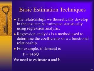
Basic Estimation Techniques. The relationships we theoretically develop in the text can be estimated statistically using regression analysis, Regression analysis is a method used to determine the coefficients of a a functional relationship. For example, if demand is P = a+bQ

Basic Estimation Techniques
E N D
Presentation Transcript
Basic Estimation Techniques • The relationships we theoretically develop in the text can be estimated statistically using regression analysis, • Regression analysis is a method used to determine the coefficients of a a functional relationship. • For example, if demand is P = a+bQ We need to estimate a and b.
Ordinary Least Squares(OLS) • Means to determine regression equation that “best” fits data • Goal is to select the line(proper intercept & slope) that minimizes the sum of the squared vertical deviations • Minimize ei2 which is equivalent to minimizing (Yi -(Y-hat)i)2
Standard Error of the Estimate • Measures variability about the regression equation • Labeled SEE • If SEE = 0 all points are on line and fit is perfect
Standard Error of the Slope • Measures theoretical variability in estimated slope - different datasets(samples) would yield different slopes
Variability in the Dependent Variable • The sum of squares of Y about its mean value is representative of the total variation in Y
Variability in the Dependent Variable • The sum of squares of Y about the regression line(Y-hat) is representative of the “unexplained” or residual variation in Y
Variability in the Dependent Variable • The sum of squares of Y-hat about Y-bar is representative of the “explained” variation in Y
Variability in the Dependent Variable • Note, TSS = ESS + RSS • If all data points are on the regression line, RSS=0 and TSS=ESS • If the regression line is horizontal, slope = 0, ESS=0 and TSS=RSS • The better the fit of the regression line to the data, the smaller is RSS
Describing Overall Fit - R2 • The coefficient of determination is the ratio of the “explained” sum of squares to the total sum of squares
Coefficient of Determination • R2 yields the percentage of variability in Y that is explained by the regression equation • It ranges between 0 and 1 • What is true if R2 = 1? • What is true if R2 = 0?
Statistical Inference • Drawing conclusions about the population based on sample information. • Hypothesis Testing • which independent variables are significant? • Is the model significant? • Estimation - point versus interval • what is the rate of change in Y per X? • what is the expected value of Y based on X
Errors in Hypotheses Testing • Type I error - rejecting the null hypothesis when it is true • Type II error - accepting the null hypothesis when it is false • Will never eliminate the possibility of error - but can control their likelihood
Structuring the Null and Alternative Hypotheses • The null hypothesis is often the reverse of what theory or logic suggest the researcher believes; it is structured to allow the data to contradict it. In the model on the effect of price on quantity demanded, the researcher would expect price to inversely impact amount purchased. Thus, the null might be that price does not effect quantity demanded or it effects it in a positive direction.
Structuring the Null and Alternative Hypotheses • Model: QA=B0+B1PA+B2Inc+B3PB+ • QA = quantity demanded of good A • PA = price of good A • Inc = Income • PB = price of good B • H0: B1 0 • HA: B1 < 0 Law of Demand expectation
H0 : 1 = 0 Reject Reject Do Not Reject /2 /2
H0 : 1 0 Reject Do Not Reject
H0 : 1 0 Do Not Reject Reject
The t-Test for the Slope • We can test the significance of an independent variable by testing the following H0 : k = 0 k = 1,2,….K HA : k 0 • Note if k = 0 a change in the kth independent variable has no impact on Y
The t-Test for the Slope • The test statistic is
T-Test Decision Rule • The critical t-value, tc, is the value that defines the boundary line separating the rejection from the do not reject region. • For a 2-tailed test if |tk| > tc, reject the null; otherwise do not reject • For a 1-tailed test if |tk| > tc and if tc has the sign implied by HA, reject the null; otherwise do not reject
F-Test and ANOVA • F-Test is used to test the overall significance of the regression or model • Analysis of Variance = ANOVA • ANOVA is based on the components of the variation in Y previously discussed - TSS, ESS, and RSS
Hypotheses for F-Test • H0: 1= 2=…..= K=0 HA: H0 is not true • Note the null suggests that all slopes are simultaneously zero and that the model would NOT be significant, ie. no independent variables are significant
Decision Rule for F-Test • If F > Fc, reject the null that the model is insignificant. Note this likely to be good news - your model appears “good” • Otherwise do not reject
Excel Output Illustration 5.3 page174-75
San Mateo Santa Barbara
Log_linear Model • Constant percentage change in dependent variable in response to a 1 percent change in an independent variable • no change in direction
Double-Log Model • Taking logs of the exponential equation yields (note this is linear in the logs)
Elasticity for Double Log Model • The elasticity of Y with respect to Xor Z for a double- log model is merely the regression coefficient or b-hat or c-hat • Thus, in a double-log model the elasticities are constant and are merely equal to the estimated regression coefficients(partial slopes).