Decision Theory
Decision Theory. (Utility based agents). Agenda. Decision making with probabilistic uncertainty in actions Decision theory (economics/business, psychology) Markov Decision Process Value Iteration Policy Iteration. General Framework. An agent operates in some given finite state space

Decision Theory
E N D
Presentation Transcript
Decision Theory (Utility based agents)
Agenda • Decision making with probabilistic uncertainty in actions • Decision theory (economics/business, psychology) • Markov Decision Process • Value Iteration • Policy Iteration
General Framework • An agent operates in some given finite state space • No explicit goal state; instead, states provide rewards (positive, negative, or null) that quantify in a single unit system what the agent gets when it visits this state (e.g., a bag of gold, a sunny afternoon on the beach, a speeding ticket, etc...) • Each action has several possible outcomes, each with some probability; sensing may also be imperfect • The agent’s goal is to plan a strategy (here, it is called a policy) to maximize the expected amount of rewards collected
Two Cases • Uncertainty in action only [The world is fully observable] • Uncertainty in both action and sensing [The world is partially observable]
Action Model • States s S • Action a: a(s) = {(s1,p1), (s2,p2), ... , (sn,pn)} probability distribution over possible successor states [ ] Markov assumption: The action model a(s) does not depend on what happened prior to reaching s
s0 A1 0.2 0.1 0.7 s1 s2 s3 Starting very simple ... • S0 describes many actual states of the real world. A1 reaches s1 in some states, s2 in others, and s3 in the remaining ones • If the agent could return to S0 many times in independent ways and if at each time it executed A1, then it would reach s1 20% of the times, s2 70% of the times, and s3 10% of the times
s0 A1 0.2 0.1 0.7 s1 s2 s3 100 50 70 rewards associated with states s1, s2, and s3 Introducing rewards ... • Assume that the agent receives rewards in some states (rewards can be positive or negative) • If the agent could execute A1 in S0 many times, the average (expected) reward that it would get is:U(S0,A1)= 100x0.2 + 50x0.7 + 70x0.1 = 20 + 35 + 7 = 62
s0 A1 A2 0.2 0.1 0.7 s1 s2 s3 100 50 70 80 ... and a second action ... • U(S0,A1) = 62 • U(S0,A2) = 78 • If the agent chooses to execute A2, it will maximize the average collected rewards 0.20.8 s4
s0 A1 A2 0.2 0.1 0.7 s1 s2 s3 100 50 70 80 ... and action costs • We may associate costs with actions, which are subtracted from the rewards • U(S0,A1) = 62 – 5 = 57 • U(S0,A2) = 78 – 25 = 53 • When in s0, the agent will now gain more on the average by executing A1 than by executing A2 -5 -25 0.20.8 s4
Juliet’s off. 5min 10min Charles’ off. 10min Conf. room A complete (but still very simple) example: Finding Juliet • A robot, Romeo, is in Charles’ office and must deliver a letter to Juliet • Juliet is either in her office, or in the conference room. Each possibility has probability 0.5 • Traveling takes 5 minutes between Charles’ and Juliet’s office, 10 minutes between Charles’ or Juliet’s office and the conference room • To perform his duties well and save battery, the robot wants to deliver the letter while minimizing the time spent in transit
States and Actions in Finding-Juliet Problem • States: • S0: Romeo in Charles’ office • S1: Romeo in Juliet’s office and Juliet here • S2: Romeo in Juliet’s office and Juliet not here • S3: Romeo in conference room and Juliet here • S4: Romeo in conference room and Juliet not here • In this example, S1 and S3 are terminal states • Actions: • GJO (go to Juliet’s office) • GCR (go to conference room) • The uncertainty in an action is directly linked to the uncertainty in Juliet’s location
-10 -5 Juliet’s off. 5min 100 100 10min Charles’ off. 10min Conf. room -10 -10 100 100 State/Action Tree s0 GJO GCR 0.5 0.5 0.5 0.5 s4 s2 s1 s3 • In this example, only the terminal states give positive rewards (say, 100) • The cost of each action (~ negative reward of reached state) is its duration GCR GJO 1.0 1.0 s1 s3
10 5 Juliet’s off. 5min 95 90 10min Charles’ off. 10min Conf. room 10 10 85 80 Forward View of Utility s0 0 GJO GCR s4 s2 s1 s3 -10 -5 • In this example, only the terminal states give positive rewards (say, 100) • The cost of each action (~ negative reward of reached state) is its duration GCR GJO s1 s3
10 5 Juliet’s off. 5min 100 100 10min Charles’ off. 10min Conf. room 10 10 100 100 Backward View of Utility s0 GJO GCR s4 s2 s1 s3 • The computation of U (utility) at each non-terminal node resembles backing up the values of an evaluation function in adversarial search GCR GJO s1 s3
10 5 Juliet’s off. 5min 100 100 10min Charles’ off. 10min Conf. room 10 10 100 100 Backward View of Rewards s0 GJO GCR s4 s2 s1 s3 • The computation of U (utility) at each non-terminal node resembles backing up the values of an evaluation function in adversarial search GCR GJO 90 90 s1 s3
10 5 Juliet’s off. 5min 100 100 10min Charles’ off. 10min Conf. room 10 10 100 100 Backward View of Utility s0 GJO GCR s4 s2 s1 s3 90 90 • The computation of U (utility) at each non-terminal node resembles backing up the values of an evaluation function in adversarial search GCR GJO 90 90 s1 s3
10 5 Juliet’s off. 5min 100 100 10min Charles’ off. 10min Conf. room 10 10 100 100 Backward View of Utility s0 U(s0,GCR) = 0.5*90+0.5*100-5 GJO GCR 85 90 U(s0,GJO) = 0.5*90+0.5*100-10 s4 s2 s1 s3 90 90 • The computation of U (utility) at each non-terminal node resembles backing up the values of an evaluation function in adversarial search GCR GJO 90 90 s1 s3
U(s0) = max{85, 90} 10 5 Juliet’s off. 5min 10min Charles’ off. 10min Conf. room 10 10 Backward View of Utility s0 90 GJO GCR 85 90 s4 s2 s1 s3 90 90 100 100 • The computation of U (utility) at each non-terminal node resembles backing up the values of an evaluation function in adversarial search • The best choice in s0 is to select GJO GCR GJO 90 90 s1 s3 100 100
Generalization • Inputs: • Initial state s0 • Action model P(s’|s,a) • Reward R(s) collected in each state s • A state is terminal if it has no successor • Starting at s0, the agent keeps executing actions until it reaches a terminal state • Its goal is to maximize the expected sum of rewards collected (additive rewards) • Assume for a while that the same state can’t be reached twice (no cycles)[finite state space finite state/action tree]
Policies • A policy(s) is a map that gives an action to take if the agent finds itself in state s • The expected sum of rewards (utility) accumulated by an agent that follows policy starting at s is • U(s) = E[t R(St)] • Where St is the random variable denoting the state that the agent will be in at time t (S0=s) • [E[X] denotes the expected value of X] • [Forward view]
Policies • A policy(s) is a map that gives an action to take if the agent finds itself in state s • The expected sum of rewards (utility) accumulated by an agent that follows policy starting at s is • U(s) = E[t R(St)] • Where St is the random variable denoting the state that the agent will be in at time t (S0=s) • [Forward view] • We want to find the policy * that maximize U(s) • Define the true utility U(s)=U*(s)
From Utility to Policies • If we knew U(s), every time the agent found itself in state s, it could simply take the action: (s) = argmaxa s’SP(s’|s,a)U(s’) • Since U(s’) measures the expected sum of collected rewards in the future state s’, it makes sense to pick the action that maximizes the expectation of U(s’) • In fact, this gives the optimal policy
Utility of a State • The utility of a state s measures its desirability: • If s is terminal:U(s) = R(s) • If s is non-terminal:U(s) = R(s) + maxaAppl(s)Σs’Succ(s,a)P(s’|s,a)U(s’) [the reward of s augmented by the expected sum of rewards collected in future states]
U(s) = R(s) + maxaAppl(s)Σs’Succ(s,a)P(s’|s,a)U(s’) Appl(s) is the set of all actions applicable to state s Succ(s,a) is the set of all possible states after applying a to s P(s’|s,a) is the probability of being in s’ after executing a in s [the reward of s augmented by the expected sum of rewards collected in future states]
Utility of a State • The utility of a state s measures its desirability: • If s is terminal:U(s) = R(s) • If s is non-terminal:U(s) = R(s) + maxaAppl(s)Σs’Succ(s,a)P(s’|s,a)U(s’) [the reward of s augmented by the expected sum of rewards collected in future states] Assume there is no cycle
U(s) = R(s) + maxaAppl(s)Ss’Succ(s,a) P(s’|s,a)U(s’)
Utility with Action Costs • U(s) = R(s) + maxaAppl(s)[-cost(a) + Σs’Succ(s,a)P(s’|s,a)U(s’)] Cost of action a + expected rewards collected in future states Bellman equation
Issues • What if the set of states reachable from the initial state is too large to be entirely generated (e.g., there is a time limit)? • How to deal with cycles (states that can be reached multiple times)?
Computation-Limited Setting • What if the set of states reachable from the initial state is too large to be entirely generated (e.g., there is a time limit)? • Expand the state/action tree to some depth h • Estimate the utilities of leaf nodes [Reminiscent of evaluation function in game trees] • Back-up utilities as described before (using estimated utilities at leaf nodes)
target robot Target-Tracking Example • The robot must keep a target in its field of view • The robot has a prior map of the obstacles • But it does not know the target’s trajectory in advance
target robot Target-Tracking Example • Time is discretized into small steps of unit duration • At each time step, each of the two agents moves by at most one increment along a single axis • The two moves are simultaneous • The robot senses the new position of the target at each step • The target is not influenced by the robot (non-adversarial, non-cooperative target)
([i,j], [u,v], t) • ([i+1,j], [u,v], t+1) • ([i+1,j], [u-1,v], t+1) • ([i+1,j], [u+1,v], t+1) • ([i+1,j], [u,v-1], t+1) • ([i+1,j], [u,v+1], t+1) right Time-Stamped States (no cycles possible) • State = (robot-position, target-position, time) • In each state, the robot can execute 5 possible actions : {stop, up, down, right, left} • Each action has 5 possible outcomes (one for each possible action of the target), with some probability distribution [Potential collisions are ignored for simplifying the presentation]
Rewards and Costs • The robot must keep seeing the target as long as possible • Each state where it does not see the target is terminal • The reward collected in every non-terminal state is 1; it is 0 in each terminal state[ The sum of the rewards collected in an execution run is exactly the amount of time the robot sees the target] • No cost for moving vs. not moving
Expanding the state/action tree ... horizon h horizon 1
Assigning rewards • Terminal states: states where the target is not visible • Rewards: 1 in non-terminal states; 0 in others • But how to estimate the utility of a leaf at horizon h? ... horizon h horizon 1
d target robot Estimating the utility of a leaf ... • Compute the shortest distance d for the target to escape the robot’s current field of view • If the maximal velocity v of the target is known, estimate the utility of the state to d/v [conservative estimate] horizon h horizon 1
Selecting the next action • Compute the optimal policy over the state/action tree using estimated utilities at leaf nodes • Execute only the first step of this policy • Repeat everything again at t+1… (sliding horizon) ... Real-time constraint: h is chosen so that a decision can be returned in unit time [A larger h may result in a better decision that will arrive too late !!] horizon h horizon 1
In this target-tracking example stamping states by time is a “trick” to avoid cycles • If the probability distribution of the target’s possible moves at each time step does not depend on past history (Markov assumption), then the best move of the robot at any time step should only depend on the robot’s and target’s current positions, not on time • To find this best move, we must remove the time stamp and handle cycles appropriately
3 square(3,2) 2 1 1 2 3 4 Robot Navigation Example • The robot (shown ) lives in a world described by a 4x3 grid of squares with square (2,2) occupied by an obstacle • A state is defined by the square in which the robot is located: (1,1) in the above figure 11 states
3 2 1 1 2 3 4 Action (Transition) Model • U brings the robot to: • (1,2) with probability 0.8 • (2,1) with probability 0.1 • (1,1) with probability 0.1 • In each state, the robot’s possible actions are {U, D, R, L} • For each action: • With probability 0.8 the robot does the right thing (moves up, down, right, or left by one square) • With probability 0.1 it moves in a direction perpendicular to the intended one • If the robot can’t move, it stays in the same square • [This model satisfies the Markov condition]
3 2 1 1 2 3 4 Action (Transition) Model • L brings the robot to: • (1,1) with probability 0.8 + 0.1 = 0.9 • (1,2) with probability 0.1 • In each state, the robot’s possible actions are {U, D, R, L} • For each action: • With probability 0.8 the robot does the right thing (moves up, down, right, or left by one square) • With probability 0.1 it moves in a direction perpendicular to the intended one • If the robot can’t move, it stays in the same square • [This model satisfies the Markov condition]
-.04 -.04 -.04 +1 3 -.04 -.04 -1 2 -.04 -.04 -.04 -.04 1 1 2 3 4 Terminal States, Rewards, and Costs • Two terminal states: (4,2) and (4,3) • Rewards: • R(4,3) = +1 [The robot finds gold] • R(4,2) = -1 [The robot gets trapped in quick sands] • R(s) = -0.04 in all other states • Actions have zero cost [actually, they are encoded in the negative rewards of non-terminal states]
0.81 0.87 0.92 +1 3 0.76 0.66 -1 2 0.71 0.66 0.61 0.39 1 1 2 3 4 State Utilities • The utility of a state s is the maximal expected amount of reward that the robot will collect from s and future states by executing some action in each encountered state, until it reaches a terminal state (infinite horizon) • Under the Markov and infinite horizon assumptions, the utility of s is independent of when and how s is reached[It only depends on the possible sequences of states after s, not on the possible sequences before s]
+1 +1 3 3 -1 -1 2 2 1 1 1 1 2 2 3 3 4 4 (Stationary) Policy • A stationary policy is a complete map P: state action • For each non-terminal state it recommends an action, independent of when and how the state is reached • Under the Markov and infinite horizon assumptions, the optimal policy P* is necessarily a stationary policy [The best action in a state does not depends on the past]
+1 +1 3 3 -1 -1 2 2 1 1 1 1 2 2 3 3 4 4 The optimal policy tries to avoid “dangerous” state (3,2) (Stationary) Policy • A stationary policy is a complete map P: state action • For each non-terminal state it recommends an action, independent of when and how the state is reached • Under the Markov and infinite horizon assumptions, the optimal policy P* is necessarily a stationary policy [The best action in a state does not depends on the past] • Finding P* is called an observable Markov Decision Problem (MDP)
+1 3 -1 2 1 1 2 3 4 Execution of Optimal Policy • Repeat: • ssensed state • If s is terminal then exit • a P*(s) • Perform a • (Reactive agent algorithm) • Let the robot executes P* many times from the same state s • Each run produces a sequence of states with some probability • Each possible sequence collects a certain amount of reward • The utility of s is the average amount of reward collected over the successive executions of P* • It is maximal over all policies
+1 +1 -1 -1 R(s) = -2 R(s) = -0.04 +1 +1 -1 -1 R(s) = -0.01 Optimal Policies for Various R(s) R(s) > 0
+1 3 -1 2 1 1 2 3 4 Defining Equations • If s is terminal: U(s) = R(s) • If s is non-terminal: U(s) = R(s) + maxaAppl(s)Ss’Succ(s,a)P(s’|a,s)U(s’) [Bellman equation] • P*(s) = argmaxaAppl(s)Ss’Succ(s,a)P(s’|a,s)U(s’)

