V10 Topologies and Dynamics of Gene Regulatory Networks

1. V10 Topologies and Dynamics of Gene Regulatory Networks Who are the players in GRNs? SILAC technology What are the kinetic rates? DREAM3 contest for network reconstruction Algorithm by team of Mark Gerstein Bioinformatics III

2. Rates of mRNA transcription and protein translation SILAC: „stable isotope labelling by amino acids in cell culture“ means that cells are cultivated in a medium containing heavy stable-isotope versions of essential amino acids. When non-labelled (i.e. light) cells are transferred to heavy SILAC growth medium, newly synthesized proteins incorporate the heavy label while pre-existing proteins remain in the light form. Parallel quantification of mRNA and protein turnover and levels. Mouse fibroblasts were pulse-labelled with heavy amino acids (SILAC, left) and the nucleoside 4-thiouridine (4sU, right). Protein and mRNA turnover is quantified by mass spectrometry and next-generation sequencing, respectively. Schwanhäuser et al. Nature 473, 337 (2011) Bioinformatics III

3. Rates of mRNA transcription and protein translation 84,676 peptide sequences were identified by MS and assigned to 6,445 unique proteins. 5,279 of these proteins were quantified by at least three heavy to light (H/L) peptide ratios Mass spectra of peptides for two proteins. Top: high-turnover protein Bottom: low-turnover protein. Over time, the heavy to light (H/L) ratios increase. Schwanhäuser et al. Nature 473, 337 (2011) Bioinformatics III

4. Protein half-lives Protein half-lives were calculated from log H/L ratios at all three time points using linear regression. The same is done to compute mRNA half-lives (not shown). Schwanhäuser et al. Nature 473, 337 (2011) Bioinformatics III

5. mRNA and protein levels and half-lives a, b, Histograms of mRNA (blue) and protein (red) half-lives (a) and levels (b). Proteins were on average 5 times more stable (9h vs. 46h) and 900 times more abundant than mRNAs and spanned a higher dynamic range. c, d, Although mRNA and protein levels correlated significantly, correlation of half-lives was virtually absent Schwanhäuser et al. Nature 473, 337 (2011) Bioinformatics III

6. Mathematical model A widely used minimal description of the dynamics of transcription and translation includes the synthesis and degradation of mRNA and protein, respectively The mRNA (R) is synthesized with a constant rate vsrand degraded proportional to their numbers with rate constant kdr. The protein level (P) depends on the number of mRNAs, which are translated with rate constant ksp. Protein degradation is characterized by the rate constant kdp. The synthesis rates of mRNA and protein are calculated from their measured half lives and levels Schwanhäuser et al. Nature 473, 337 (2011) Bioinformatics III

7. Computed transcription and translation rates Average cellular transcription rates predicted by the model spanned two orders of magnitude. The median is about 2 mRNA molecules per hour (b). An extreme example is Mdm2 with more than 500 mRNAs per hour The median translation rate constant is about 40 proteins per mRNA per hour Calculated translation rate constants are not uniform Schwanhäuser et al. Nature 473, 337 (2011) Bioinformatics III

8. Maximal translation constant Abundant proteins are translated about 100 times more efficiently than those of low abundance Translation rate constants of abundant proteins saturate between approximately 120 and 240 proteins per mRNA per hour. The maximal translation rate constant in mammals is not known. The estimated maximal translation rate constant in sea urchin embryos is 140 copies per mRNA per hour, which is surprisingly close to the prediction of this model. Schwanhäuser et al. Nature 473, 337 (2011) Bioinformatics III

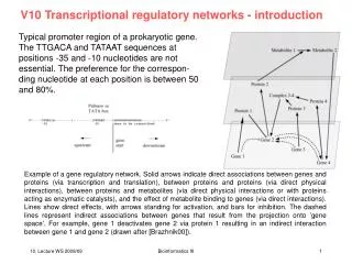
9. Mathematical reconstruction of Gene Regulatory Networks DREAM: Dialogue on Reverse Engineerging Assessment and Methods Aim: systematic evaluation of methods for reverse engineering of network topologies (also termed network-inference methods). Problem: correct answer is typically not known for real biological networks Approach: generate synthetic data Marbach et al. PNAS 107, 6286 (2010) Gustavo Stolovitzky/IBM Bioinformatics III

10. Generation of Synthetic Data Transcriptional regulatory networks are modelled consisting of genes, mRNA, and proteins. The state of the network is given by the vector of mRNA concentrations x and protein concentrations y. We model only transcriptional regulation, where regulatory proteins (TFs) control the transcription rate (activation) of genes (no epigenetics, microRNAs etc.). The gene network is modeled by a system of differential equations where mi is the maximum transcription rate, rithe translation rate, λiRNAand λiProt are the mRNA and protein degradation rates and fi(.) is the so-called input function of gene i. Marbach et al. PNAS 107, 6286 (2010) Bioinformatics III

11. The input function fi() The input function describes the relative activation of the gene, which is between 0 (the gene is shut off) and 1 (the gene is maximally activated), given the transcription-factor (TF) concentrations y. We assume that binding of TFs to cis-regulatory sites on the DNA is in quasi-equilibrium, since it is orders of magnitudes faster than transcription and translation. In the most simple case, a gene i is regulated by a single TF j. In this case, its promoter has only two states: either the TF is bound (state S1) or it is not bound (state S0). The probability P(S1) that the gene i is in state S1 at a particular moment is given by the fractional saturation, which depends on the TF concentration yj where kij is the dissociation constant and nij the Hill coefficient (formula not derived here). Marbach et al. PNAS 107, 6286 (2010) Bioinformatics III

12. The input function fi() P(S1) is large if the concentration of the TF j is large and if the dissociation constant is small (strong binding). The bound TF activates or represses the expression of the gene. In state S0 the relative activation is α0 and in state S1 it is α1. Given P(S1) and its complement P(S0) , the input function fi(yj) is obtained, which computes the mean activation of gene i as a function of the TF concentration yj Marbach et al. PNAS 107, 6286 (2010) Bioinformatics III

13. The input function fi() This approach can be used for an arbitrary number of regulatory inputs. A gene that is controlled by N TFs has 2N states: each of the TFs can be bound or not bound. Thus, the input function for N regulators would be Marbach et al. PNAS 107, 6286 (2010) Bioinformatics III

14. Synthetic gene expression data Gene knockouts were simulated by setting the maximum transcription rate of the deleted gene to zero, knockdowns by dividing it by two. Time-series experiments were simulated by integrating the networks using different initial conditions. For the networks of size 10, 50, and 100, they provided 4, 23, and 46 different time series, respectively. For each time series, a different random initial condition was used for the mRNA and protein concentrations. Each time series consisted of 21 time points. Trajectories were obtained by integrating the networks from the given initial conditions using a Runge-Kutta solver. White noise with a standard deviation of 0.05 was added after the simulation to the generated gene expression data. Marbach et al. PNAS 107, 6286 (2010) Bioinformatics III

15. Synthetic networks The challenge was structured as three separate subchallenges with networks of 10, 50, and 100 genes, respectively. For each size, five in silico networks were generated. These resembled realistic network structures by extracting modules from known transcriptional regulatory network for Escherichia coli (2x) and for yeast (3x). Example network E.coli Example network yeast Marbach et al. PNAS 107, 6286 (2010) Bioinformatics III

16. Evaluation of network predictions (A) The true connectivity of one of the benchmark networks of size 10. (C) The network prediction is evaluated by computing a P-value that indicates its statistical significance compared to random network predictions. (B) Example of a prediction by the best-performer team. The format is a ranked list of predicted edges, represented here by the vertical colored bar. The white stripes indicate the true edges of the target network. A perfect prediction would have all white stripes at the top of the list. Inset shows the first 10 predicted edges: the top 4 are correct, followed by an incorrect prediction, etc. The color indicates the precision at that point in the list. E.g., after the first 10 predictions, the precision is 0.7 (7 correct predictions out of 10 predictions). Marbach et al. PNAS 107, 6286 (2010) Bioinformatics III

17. Similar performance on different network sizes The method by Yip et al. gave the best results for all 3 network sizes. Marbach et al. PNAS 107, 6286 (2010) Bioinformatics III

18. Error analysis Left: 3 typical errors made in predicted networks. We will now discuss the best-performing method by Yip et al. Only this method gives stable results independent of the indegree of the target (right) Marbach et al. PNAS 107, 6286 (2010) Bioinformatics III

19. Synthetic networks Best performing team in DREAM3 contest Applied a simple noise model and linear and sigmoidal ODE models. Predictions from the 3 models were combined. Mark Gerstein/Yale Yip et al. PloS ONE 5:e8121 (2010) Bioinformatics III

20. Cumulative distribution function The cumulative distribution function (CDF) describes the probability that a real-valued random variable X with a given probability distribution will be found at a value less than or equal to x. The complementary cumulative distribution function (ccdf) or simply the tail distribution addresses the opposite question and asks how often the random variable is above a particular level. It is defined as Different normal distributions CDF of the normal distribution www.wikipedia.org Bioinformatics III

21. Noise model • If we were given: • xab : observed expression level of gene a in deletion strain of gene b, and • xawt*: real expression level of gene a in wild type xawt* (without noise) • we would like to know whether the deviation xab - xawt* is merely due to noise. • Need to know the variance σ2 of the Gaussian, • assuming the noise is non systematic so that the mean μ is zero. • Later, we will discuss the fact that xawt*: is also subject to noise so that we are • only provided with the observed level xawt . Yip et al. PloS ONE 5:e8121 (2010) Bioinformatics III

22. Noise model The probability for observing a deviation at least as large as xab - xawt* due to random chance is where Φ is the cumulative distribution function of the standard Gaussian distribution. The deviation is taken relative to the width (standard dev.) of the Gaussian which describes the magnitude of the „normal“ spread in the data. 1 - CDF measures the area in the tail of the distribution. The factor 2 accounts for the fact that we have two tails left and right. The complement of this is the probability that the deviation is due to a real (i.e. non-random) regulation event. Yip et al. PloS ONE 5:e8121 (2010) Bioinformatics III

23. Noise model • One can then rank all the gene pairs (b,a) in descending order of pba. • For this we first need to estimate σ2 from the data. • Two difficulties. • the set of genes a not affected by the deleted gene b is unknown. This is exactly what we are trying to learn from the data. • the observed expression value of a gene in the wild-type strain, xawt, is also subjected to random noise, and thus cannot be used as the gold-standard reference point xawt* in the calculations • Use iterative procedure to progressively refine estimation of pba. Yip et al. PloS ONE 5:e8121 (2010) Bioinformatics III

24. Noise model We start by assuming that the observed wild-type expression levels xawt are reasonable rough estimates of the real wild type expression levels xawt*. For each gene a, our initial estimate for the variance of the Gaussian noise is set as the sample variance of all the expression values of a in the different deletion strains b1 - bn. Repeat the following 3 steps for a number of iterations: (1). Calculate the probability of regulation pba for each pair of genes (b,a) based on the current reference points xawt. Then use a p-value of 0.05 to define the set of potential regulation: if the probability for the observed deviation from wild type of a gene a in a deletion strain b to be due to random chance only is less than 0.05, we treat ba as a potential regulation. Otherwise, we add (b,a) to the set P of gene pairs for refining the error model. Yip et al. PloS ONE 5:e8121 (2010) Bioinformatics III

25. Noise model (2) Use the expression values of the genes in set P to re-estimate the variance of the Gaussian noise. (3) For each gene a, we re-estimate its wild-type expression level by the mean of its observed expression levels in strains in which the expression level of a is unaffected by the deletion After the iterations, the probability of regulation pba is computed using the final estimate of the reference points xawtand the variance of the Gaussian noise σ2 . Yip et al. PloS ONE 5:e8121 (2010) Bioinformatics III

26. Learning ODE models from perturbation time series data For time series data after an initial perturbation, we use differential equations to model the gene expression rates. The general form is as follows: with xi : expression level of gene i , fi (…): function that explains how the expression rate of gene i is affected by the expression level of all the genes in the network, including the level of gene i itself. Yip et al. PloS ONE 5:e8121 (2010) Bioinformatics III

27. Learning ODE models from perturbation time series data Various types of function fi have been proposed. We consider two of them. The first one is a linear model ai0 : basal expression rate of gene i in the absence of regulators, aii : decay rate of mRNA transcripts of i, S : set of potential regulators of i (we assume no self regulation, so i not element of S). For each potential regulator j in S, aij explains how the expression of i is affected by the abundance of j. A positive aij indicates that j is an activator of i , and a negative aij indicates that j is a suppressor of i . The linear model contains Ι S Ι + 2 parameters aij. Yip et al. PloS ONE 5:e8121 (2010) Bioinformatics III

28. Learning ODE models from perturbation time series data The linear model assumes a linear relationship between the expression level of the regulators and the resulting expression rate of the target. But real biological regulatory systems seem to exhibit nonlinear characteristics. The second model assumes a sigmoidal relationship between the regulators and the target bi1 : maximum expression rate of i , bi2 : its decay rate The sigmoidal model contains Ι S Ι + 3 parameters. Try 100 random initial values and refine parameters by Newton minimizer so that the predicted expression time series give the least squared distance from the real time series. Score: negative squared distance Yip et al. PloS ONE 5:e8121 (2010) Bioinformatics III

29. Learning ODE models from perturbation time series data • Batch 1 contains the most confident predictions: all predictions with probability of regulation (pba > 0.99 according to the noise model learned from homozygous deletion data • Batch 2: all predictions with a score two standard deviations below the average according to all types (linear AND sigmoidal) of differential equation models learned from perturbation data • Batch 3: all predictions with a score two standard deviations below the average according to all types of guided differential equation models learned from perturbation data, where the regulator sets contain regulators predicted in the previous batches, plus one extra potential regulator • Batch 4: as in batch 2, but requiring the predictions to be made by only one type (linear OR sigmoidal) of the differential equation models as opposed to all of them. • Batch 5: as in batch 3, but requiring the predictions to be made by only one type of the differential equation models as opposed to all of them • Batch 6: all predictions with pba > 0.95 according to both the noise models learned from homozygous and heterozygous deletion data, and have the same edge sign predicted by both models • Batch 7: all remaining gene pairs, with their ranks within the batch determined by their probability of regulation according to the noise model learned from homozygous deletion data Yip et al. PloS ONE 5:e8121 (2010) Bioinformatics III

30. Learning ODE models from perturbation time series data Yip et al. PloS ONE 5:e8121 (2010) Bioinformatics III

31. Learning ODE models from perturbation time series data Interpretation: A network with 10 nodes has 10 x 9 possible edges Batch 1 already contains many of the correct edges (7/11 – 8/22). The majority of the high-confidence predictions are correct (7/11 – 8/12). Batch 7 contains only 1 correct edge for the E.coli-like network, but 9 or 10 correct edges for the Yeast-like network. Yip et al. PloS ONE 5:e8121 (2010) Bioinformatics III

32. Learning ODE models from perturbation time series data Not all regulation arcs can be detected from deletion data (middle): Left: G7 is suppressed by G3, G8 and G10 Right: G8 and G10 have high expression levels in wt. Middle: removing the inhibition by G3 therefore only leads to small increase of G7 which is difficult to detect. However the right panel suggests that the increased expression of G7 over time is anti-correlated with the decreased level of G3  This link was detected by the ODE-models in batch 2 Yip et al. PloS ONE 5:e8121 (2010) Bioinformatics III

33. Learning ODE models from perturbation time series data Another case: Left: G6 is activated by G1 and suppressed by G5. G1 also suppresses G5. G1 therefore has 2 functions on G6. When G1 is expressed, deleting G5 (middle) has no effect. Right: G6 appears anti-correlated to G1. Does not fit with activating role of G1. But G5 is also anti-correlated with G6  evidence for inhibitory role of G5. Yip et al. PloS ONE 5:e8121 (2010) Bioinformatics III

34. Summary : deciphering GRN topologies is hard GRN networks are hot topic. They give detailed insight into the circuitry of cells. This is important for understanding the molecular causes e.g. of diseases. New data are constantly appearing. The computational algorithms need to be adapted. Perturbation data (knockouts and time series following perturbations) are most useful for mathematic reconstruction of GRN topologies. Yip et al. PloS ONE 5:e8121 (2010) Bioinformatics III