Download
1 / 29
290 likes | 434 Vues
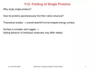
V12: Folding of Single Proteins. Why study single proteins? How do proteins spontaneously find their native structure? Theoretical studies overall downhill funnel-shaped energy surface. Surface is complex and rugged folding behavior of individual molecules may differ widely!.

E N D
V12: Folding of Single Proteins Why study single proteins? How do proteins spontaneously find their native structure? Theoretical studies overall downhill funnel-shaped energy surface. Surface is complex and rugged folding behavior of individual molecules may differ widely! Optimization, Energy Landscapes, Protein Folding
V2: NMR-Daten für Faltung von Lysozym Man findet zwei Faltungs- pfade. Der gelbe ist schnell, der grüne langsam. Dobson, Karplus, Angew. Chemie Int. Ed. 37, 868 (1998) Optimization, Energy Landscapes, Protein Folding
Folding of Single Proteins: experimental realisation Reversible folding/unfolding transitions of single protein molecules can be studied at equilibrium. Choose experimental conditions under which each protein molecules spends (on average) an equal amount of time on the two sides of the folding barrier. Monitor e.g. FRET signal between fluorescent probes attached to 2 ends of molecule. Optimization, Energy Landscapes, Protein Folding
Using FRET to Study Folding of Single Proteins Schematic structures of protein and polyproline helices labelled with donor (Alexa 488) and acceptor (Alexa 594) dyes. a, Folded CspTm, a 66-residue, five-stranded -barrel protein; b, unfolded CspTm; c, (Pro)6; and d, (Pro)20 . A blue laser excites the green-emitting donor dye, which can transfer excitation energy to the red-emitting acceptor dye at a rate that depends on the inverse sixth power of the interdye distance In each case, the functional form of the FRET efficiency E versus distance (blue curve) is shown, as well as a representation of the probability distribution of distances between donor and acceptor dyes, P (red curve). Schuler et al. Nature 419, 743 (2002) Optimization, Energy Landscapes, Protein Folding
FRET efficiencies for single molecules Dependence of the means and widths of the measured FRET efficiency (Eapp) on the concentration of GdmCl. a, Eapp for (Pro)20. b , Single molecule mean values (filled circles), ensemble FRET efficiencies (open circles), and associated two-state fit (unbroken curve) for CspTm . Dotted curve: third-order polynomial fit to the unfolded protein data that was matched (dashed curve) to the ensemble data between 4 and 6 M GdmCl. Schuler et al. Nature 419, 743 (2002) Optimization, Energy Landscapes, Protein Folding
Influence of Protein Dynamics on Width Two limiting cases for polypeptide dynamics in experiments on freely diffusing molecules. a , If the end-to-end distance of the protein does not change during the observation period in the illuminated volume (blue), then the distribution of transfer efficiencies reflects the equilibrium end-to-end distance distribution of the molecules and consequently results in a very broad probability distribution of FRET efficiencies, shown here for a gaussian chain (red curve). b, If the molecule reconfigures fast relative to the time it takes to diffuse through the illuminated volume, then the FRET efficiency averages completely and is the same for every molecule. Schuler et al. Nature 419, 743 (2002) Optimization, Energy Landscapes, Protein Folding
Estimate folding barrier Upper limit for reconfiguration time in unfolded state: 0 = 25 s. Ensemble folding time 12 ms. Use Kramers equation Lower limit for free energy barrier of folding: 4 kT. Upper bound: reconfiguration time of gaussian chain: 11 kT Optimization, Energy Landscapes, Protein Folding
Limitation of previous study Free diffusion experiments can only be used to examine states that are substantially populated at equilibrium. Optimization, Energy Landscapes, Protein Folding
Folding Studies near Native Conditions Microfluidic mixer. (A) Channel pattern and photograph of mixing region as seen through the microscope objective and bonded coverslip. Solutions containing protein, denaturant, and buffer were driven through the channels with compressed air. Arrows indicate the direction of flow. (B) View of the mixing region. Computed denaturant concentration is indicated by color. The laser beam (light blue) and collected fluorescence (yellow) are shown 100 µm from the center inlet. (C) Cross section of the mixing region. Actual measurements were made at distances 100 µm from the center inlet channel. Because the flow velocity at the vertical center of the observation channel is about 1 µm ms-1, this corresponds to times 0.1 s. Lipman et al. Science 301, 1233 (2002) Optimization, Energy Landscapes, Protein Folding
Folding of Membrane Proteins (A) Histograms of measured FRET efficiency, Em, during folding. (Top) The Em distribution at equilibrium before mixing. The vertical redline indicates the mean value for Em in the unfolded state after mixing. Measurements of Em were taken (typically for 30 minutes) at various distances from the mixing region and thus at various times after the change in GdmCl concentration. (B) Comparison of single-molecule and ensemble folding kinetics. The decrease in donor fluorescence from stopped-flow experiments is shown in green. Single-molecule data are represented by filled circles, with a corresponding single exponential fit (black). The fit to the single-molecule data has a rate constant of 6.6 ± 0.8 s-1, in agreement with the result from ensemble measurements (5.7 ± 0.4 s-1). Lipman et al. Science 301, 1233 (2002) Optimization, Energy Landscapes, Protein Folding
Unfolding of CspTM in GdmCl Dependence of (A) the mean values and (B) peak widths () of Em histograms for unfolded Csp as a function of GdmCl concentration. Peak widths are standard deviations of Gaussian fits. The colored region indicates the range of denaturant concentrations where reliable data cannot be obtained from corresponding equilibrium experiments. even though there is significant compactification of U between 6 M and 0.5 M GdmCl, there is no increase in the reconfiguration time. Schuler et al. Nature 419, 743 (2002) Optimization, Energy Landscapes, Protein Folding
Folding of single adenylate kinase molecules Challenges of studies on single molecules: find a way to restrict the molecules spatially such that temporal folding trajectories can be measured without modifying the conformational dynamics of the protein. - such modification may result e.g. from immobilizing the protein on a surface. - technique used here: trap single molecules in surface-tethered unilamellar lipid vesicles. The vesicles ( = 120 nm) are much larger than the proteins ( = 5 nm) so they allow the proteins to diffuse freely. Gilad Haran, Weizman Institute Optimization, Energy Landscapes, Protein Folding
Folding of single adenylate kinase (AK) molecules Ribbon representation of the structure of AK from E. coli. Positions 73 and 203 (labeled by acceptor and donor fluorophores) are marked with arrows. Folding behavior of AK: not a simple two-state folder; at least one intermediate along folding path. Ensemble folding time ca. 4 min. Rhoades et al. PNAS 100, 3197 (2003) Optimization, Energy Landscapes, Protein Folding
Verification that AK molecules don’t interact with wall (A and B) Distributions of average fluorescence polarization values of single AK molecules labeled with the donor only obtained after excitation with circularly polarized light. The distribution shown in A is for molecules trapped in vesicles at 0.4 M Gdn•HCl, and the one shown in B is for molecules adsorbed directly on glass. The very narrow width of the polarization distributions of vesicle-trapped molecules, compared with the width of the distribution of glass-adsorbed molecules, indicates freedom of rotation of the trapped molecules. (C) A typical time-dependent fluorescence polarization trajectory of a single AK molecule labeled with the donor only and trapped in a lipid vesicle. The vertically polarized (IV) and horizontally polarized (IH) components of the fluorescence are shown in gray and black, respectively. (D) The fluorescence polarization calculated from the data in C. The lack of any long-term jumps in the polarization indicates that this protein molecule does not become static (e.g., due to adsorption on the vesicle wall) for any considerable amount of time. Rhoades et al. PNAS 100, 3197 (2003) Optimization, Energy Landscapes, Protein Folding
FRET distributions of AK in vesicles under native and midtransition conditions (A and B) Distributions of EET values obtained from single-molecule trajectories of labeled AK molecules trapped in vesicles under native and denaturing (2 M Gdn•HCl) conditions. The distributions are essentially unimodal, and their average values, 0.8 and 0.14, are close to the ensemble values. (C) Distribution of EET values obtained from single-molecule trajectories of encapsulated AK molecules prepared in 0.4 M Gdn•HCl (near midtransition conditions) that showed folding/unfolding transitions. The distribution can be roughly divided into two subdistributions, one due to the "denatured" ensemble, with EET values < 0.45, and one due to the "folded" ensemble, with EET values larger than that value, as illustrated by the black lines (Gaussian fits). The distribution of FRET efficiencies of all the trajectories measured for molecules in 0.4 M Gdn•HCl (data not shown) has peaks at the same values as the distribution made from molecules that only showed transitions (C), with a greater proportion of the distribution in the folded ensemble. Additionally, the average value of this single-molecule distribution (0.6) matches quite well with the measured ensemble value. Rhoades et al. PNAS 100, 3197 (2003) Optimization, Energy Landscapes, Protein Folding
Observation of heterogenous folding pathways (A and C) Time traces of individual vesicle-trapped AK molecules under midtransition conditions with the acceptor signal in red and the donor in green. (B and D) EET trajectories calculated from the signals in A and C, respectively. In A and B several transitions occur between states that are essentially within the "folded" ensemble, whereas in C and D a single transition takes the molecule from the folded to the "denatured" ensemble. Note that transitions can be strictly recognized by an anticorrelated change in the donor and acceptor fluorescence intensities as opposed to uncorrelated fluctuations sometimes appearing in one of the signals. Rhoades et al. PNAS 100, 3197 (2003) Optimization, Energy Landscapes, Protein Folding
Characterize folding/unfolding transitions (A) Map of folding/unfolding transitions obtained from single-molecule trajectories. Each point represents the final vs. initial FRET efficiency for one transition. The line is drawn to distinguish folding and unfolding transitions; above the line are folding transitions (efficiency increases), and below the line are unfolding transitions (efficiency decreases). (B) Distribution of transition sizes (i.e., final minus initial efficiencies) as obtained from the map in A. The two branches of the distribution represent unfolding and folding transitions, respectively. The overall similarity of the shape of the two branches indicates uniform sampling of the energy landscape. They both peak at a low efficiency value, signifying a preference for small-step transitions. Rhoades et al. PNAS 100, 3197 (2003) Optimization, Energy Landscapes, Protein Folding
Interpretation - large spread of transitions, can essentially start and end at any value of the FRET efficiency - there is a preference for steps that change EET by 0.2-0.3 AK molecules do not typically change from a fully folded to a fully unfolded conformation in one step. Rather, they jump through several intermediate steps. Unfortunately, slow folding dynamics of AK does not allow to measure folding/unfolding times directly from single-molecule trajectories. Rhoades et al. PNAS 100, 3197 (2003) Optimization, Energy Landscapes, Protein Folding
Slow Transitions and the Role of Correlated Motion Time-dependent signals from single molecules showing slow folding or unfolding transitions. (A) Signals showing a slow folding transition starting at 0.5 sec and ending at 2 sec. The same signals display a fast unfolding transition as well (at 3 sec). (B) EET trajectory calculated from the signals in A. (C) The interprobe distance trajectory showing that the slow transition involves a chain compaction by only 20%. The distance was computed from the curve in B by using a Förster distance (R0) of 49 Å. (D–F) Additional EET trajectories demonstrating slow transitions. Rhoades et al. PNAS 100, 3197 (2003) Optimization, Energy Landscapes, Protein Folding
Interpretation - In contrast to the fast intrinsic dynamics of the cold-shock protein, AK molecules show quite slow transitions. A compactation by only 20% may take as much as 1.5 s. - occurrence of transitions showing a slow, gradual change of EET indicates directed motion on energy landscape, possibly slowed down by local traps. highly correlated, non-Markovian chain dynamics? slow transition may also be result of slow growth of a folding nucleus - in the same molecule both fast and slow transitions appear. The slow transitions are not preceded by a fast jump. Enthalpic barriers very fast transition/jump, even on single molecule level. Entropic barriers diffusion through large # of local states Rhoades et al. PNAS 100, 3197 (2003) Optimization, Energy Landscapes, Protein Folding
Monitor Folding Trajectories of Single Proteins by AFM Use single-molecule AFM technique in the „force-clamp“ mode where a constant force is applied to a single polyprotein (here: typically nine repeats of ubiquitin). - monitor probabilistic unfolding of ubiquitin = stepwise elongations Fernandez and Li, Science 303, 1674 (2004) Optimization, Energy Landscapes, Protein Folding
Folding pathway of ubiquitin (A) The end-to-end length of a protein as a function of time. (B) The corresponding applied force as a function of time. The inset in (A) shows a schematic of the events that occur at different times during the stretchrelaxation cycle (numbered from 1 to 5). zp, piezoelectric actuator displacement; Lc, contour length. The length of the protein (in nanometers) evolves in time as it first extends by unfolding at a constant stretching force of 122 pN. This stage is characterized by step increases in length of 20 nm each, marking each ubiquitin unfolding event, numbered 1 to 3. The first unfolding event (1) occurred very close to the beginning of the recording and therefore it is magnified with a logarithmic time scale (blue inset) with the length dimension plotted at half scale. Upon quenching the force to 15 pN, the protein spontaneously contracted, first in a steplike manner resulting from the elastic recoil of the unfolded polymer (4), and then by a continuous collapse as the protein folds (5). The complex time course of this collapse in the protein’s length reflects the folding trajectory of ubiquitin at a low stretching force. Fernandez and Li, Science 303, 1674 (2004) Optimization, Energy Landscapes, Protein Folding
Verification To confirm that our polyubiquitin had indeed folded, at 14 s we stretched again back to 122 pN (B). The initial steplike extension is the elastic stretching of the folded polyubiquitin. Afterward, we observed steplike extension events of 20 nm each, corresponding to the unfolding of the ubiquitin proteins that had previously refolded. After these unfolding events, the length of the polyubiquitin is the same as that measured before the folding cycle began (3). Fernandez and Li, Science 303, 1674 (2004) Optimization, Energy Landscapes, Protein Folding
folding includes several discrete processes Folding is characterized by a continuous collapse rather than by a discrete all-or-none process. (A) and (B) show typical recordings of the time course of the spontaneous collapse in the end-to-end length of an unfolded polyubiquitin, observed after quenching to a low force. (A) Four distinct stages can be identified. The first stage is fast and we interpret it as the elastic recoil of an ideal polymer chain (see magnified trace in the top inset). The next three stages are marked by abrupt changes in slope and correspond to the folding trajectory of ubiquitin. These stages can be distinguished by their different slopes. Stages 2 and 3 always show peak-to-peak fluctuations in length of several nanometers. The rapid final contraction of stage 4 marks the end of the folding event. This final collapse stage is not instantaneous, as can be seen on the magnified trace in the lower inset. We measure the total duration of the collapse, t , from the beginning of the quench until the end of stage 4. Fernandez and Li, Science 303, 1674 (2004) Optimization, Energy Landscapes, Protein Folding
Length distribution of protein (B) The folding collapse is marked by large fluctuations in the length of the protein. These fluctuations greatly diminish in amplitude after folding is complete. The inset at the top is a record of the end-to-end fluctuations of the protein before the quench (region I), during the folding collapse (region II), and after folding was completed (region III). The fluctuations were obtained by measuring the residual from linear fits to the data (red dotted lines). Fernandez and Li, Science 303, 1674 (2004) Optimization, Energy Landscapes, Protein Folding
The duration of the folding collapse in force dependent We show four different traces from ubiquitin chains for which we observed seven unfolding events (recorded at 100 to 120 pN) before relaxing the force. Hence, the unfolded length of all these recordings is comparable. (A) In the first recording, the force was quenched to 50 pN (downward arrow). An instantaneous elastic recoil was observed. However, the ubiquitin chain fails to fold, as evidenced by ist constant length at this force. Upon restoration of a high stretching force (120 pN, upward arrow), the ubiquitin chain is observed to elastically extend back to its fully unfolded length. (B and C) Recordings similar to that shown in (A) (seven initial unfolding events), in which the force was quenched further down to 35 pN. In contrast to (A), the length of the ubiquitin chain was observed to spontaneously contract to the folded length. In (B), the folded ubiquitin chain was observed to unfold partially at the low force, whereas in (C) it remains folded until the high stretching force is restored (upward arrow). Several unfolding events mark this last stage, bringing the ubiquitin chain back to its unfolded length. (D) A case in which the force was quenched even further down to 23 pN. In this case, the folding collapse was completed in much less time (inset), clearly showing that the probability of observing a folding event as well as its duration is strongly force dependent. Fernandez and Li, Science 303, 1674 (2004) Optimization, Energy Landscapes, Protein Folding
Duration of folding collapse depends onprotein length and on magnitude of quence The duration of the spontaneous collapse of an unfolded ubiquitin chain (t; Fig. 2A) depends on the total contour length of the mechanically unfolded polypeptide (A) and on the magnitude of the stretching force during refolding (B). (A) Three sets of recordings grouped by force range and plotted against their contour length. The solid lines are linear fits to each set of data. To observe the force dependency we grouped the data from (A) at the highest range of contour lengths for which the effect of the force is most evident (150 to 200 nm). We observed that the duration of the folding collapse is exponentially dependent on the force (B). Fernandez and Li, Science 303, 1674 (2004) Optimization, Energy Landscapes, Protein Folding
Protein length as a function of time Two recordings of protein length (nm) as a function of time, showing the folding trajectory of a single ubiquitin. As before, stretching at a high force (100 pN) is followed by a quench to a low force of 26 pN that lasts 8 s, followed by restoration of the high stretching force up to 100 pN (bottom trace). In both cases, a single ubiquitin was observed to unfold at 100 pN. After the quench, the proteins undergo a spontaneous collapse into the folded state. Upon restretching, the folded ubiquitin is observed to elastically extend back to its folded length at 100 pN and then to unfold (second recording) . Discrete fluctuations of several nanometers can be observed shortly before the final folding contraction. The final contraction occurred much faster than the previous stage; however, it had a finite rate (insets). Fernandez and Li, Science 303, 1674 (2004) Optimization, Energy Landscapes, Protein Folding
Conclusions AFM technique allows direct monitoring of the folding pathway of single proteins. Ubiquitin folding occurs through a series of continuous stages that cannot be easily represented by state diagrams. By studying how the folding trajectories respond to a variety of physico-chemical conditions, mutagenesis, and protein engineering, we may begin to identify the physical phenomena underlying each stage in these folding trajectories. Fernandez and Li, Science 303, 1674 (2004) Optimization, Energy Landscapes, Protein Folding