Download
1 / 63
690 likes | 1.09k Vues
8. The Classification of Stellar Spectra Goals : 1. Gain a working familiarity with the primary spectral types and luminosity classes of stars with regard to strengths of specific spectral lines in stellar spectra.

E N D
8. The Classification of Stellar Spectra Goals: 1. Gain a working familiarity with the primary spectral types and luminosity classes of stars with regard to strengths of specific spectral lines in stellar spectra. 2. Become familiar with the Boltzmann and Saha equations and how they are used with stellar spectra to establish surface temperatures and luminosities for individual stars. 3. Link a knowledge of stellar temperatures and luminosities to the location of stars in the Hertzsprung-Russell diagram.
History Stellar spectra were observed and recorded long before the field of spectroscopy had fully developed. Prior to the laboratory identification of spectral lines at specific wavelengths with certain elements, some method of classifying stellar spectra was desirable. The hydrogen Balmer line sequence was recognized from the earliest such studies, and so the earliest classification scheme of any duration was a Harvard scheme developed by Pickering and Fleming based upon photographically-recorded blue-green spectra in the λ3900–5000 Å region that designated stars according to a letter sequence A, B, C, D,... based upon the decreasing strength of the hydrogen Balmer lines visible (type A having the strongest lines). Pickering and Annie Jump Cannon later revised the scheme according to information gleaned from atomic physics, which allowed one to establish element identification and degree of excitation or ionization for specific elements. The revised scheme eliminated certain redundant types and reordered the types in a logical sequence: O, B, A, F, G, K, M being a sequence in order of decreasing surface temperature.
The arrangement of spectral types in the Harvard scheme was subdivided numerically into finer temperature subtypes, such as B0, B2, B3, B5… A0, A2, A3, A5… etc. Note that not all spectral subtypes were used; types B1 and B4, among others, simply did not exist. The O-type stars were subdivided differently, i.e. Oa, Ob, Oc, Od, and Oe, in order to avoid confusion with an alternate classification scheme of that era. A major accomplishment in subsequent years was the classification of all stars brighter than ~10th magnitude photographic by Annie Jump Cannon from objective prism plates taken at observatories operated by the Harvard College Observatory. The resulting Henry Draper Catalogue and Extension (HD and HDE) is still used today.
Special designations were also developed for stars having peculiar spectral properties, namely: c = narrow lines (typical of supergiant stars) g = giant spectrum d = dwarf (main-sequence) spectrum pec = peculiar spectrum (also abbreviated to p) k = interstellar (sharp) Ca II K-line present pq = nova-like spectrum (broad emission blends) . e = emission lines present (the letter "f" was used to designate emission for O stars) ev = variable emission v = variable spectrum (as, for example, in a pulsating star) n = wide and diffuse (nebulous) spectral lines (now attributed to rapid rotation) nn = very diffuse spectral lines (for very rapid rotation) s = sharp lines (generally resulting from a very low projected rotational velocity)
Morgan-Keenan (MK) System The MK classification scheme is a refinement of the original Harvard system of stellar classification that includes a designation for the star’s luminosity as well as its temperature. The scheme went through an initial stage with a paper by Morgan, Keenan, and Kellerman (1943, called the MKK scheme), and was later revised by Morgan and Keenan (see Johnson & Morgan 1953, ApJ, 117, 313) to the present MK scheme. Later modifications include more recent MK dagger types, denoted MK†, and spectral subtypes and designations added by Nolan Walborn, Morgan's last graduate student. William Wilson Morgan 1906-1995
The MK scheme includes the temperature subtypes of the Harvard scheme, with additions to fill out the temperature subclasses detectable at the dispersion (~100 Å/mm) used for MK classification, e.g. B0, B0.5, B1… B9, B9.5, A0, A … etc. The O-type stars were reclassified numerically, the original temperature ordering becoming O6, O7, O8, O9, O9.5, B0. Luminosity classes were added using the Saha ionization law, although the original scheme was an empirical system based upon the observable spectral features of similar-temperature stars having known absolute magnitudes (measurable parallaxes and members of clusters and associations). Temperature subtypes and luminosity classes were established from specific line ratios determined from stellar spectra. The luminosity types used are: Ia = luminous supergiants (0 designates hypergiants) Ib = less luminous supergiants II = bright giants III = giants IV = subgiants V = dwarfs (main-sequence stars)
Interpolated luminosity classes are also used, such as IV-V, II-III, etc. Provisions were also made in the original scheme for subdwarfs (= VI) and white dwarfs (= VIII), but those classes never became popular. Subdwarfs are now recognized as metal-poor stars that are difficult to classify in any case, and white dwarfs are degenerate stars (D) that have since been given their own classification scheme. The original MK scheme has been improved upon by Morgan's students, such as Nolan Walborn, and by students of their students (e.g. Richard Gray). The result has been the extension of the temperature sequence for O stars to subtypes O3, O4, and O5, and a luminosity classification for O-type stars based upon their degree of "Of-ness," i.e. type f are class I, type (f) are class III, and type ((f)) are classes IV and V. Abt has done a lot of work classifying the Ap stars (A stars showing anomalous intensities of Mg, Si, Eu, and the rare earths Sr, Cr, etc.) and Am stars (metallic line strong for the strength of Ca K), and such stars are now recognized as being representative of the need for a third parameter, such as chemical composition, in the system.
MK Classification Criteria New sequence: OBAFGKMLT Atlas spectra shown on subsequent pages as they appear on photographic spectrograms.
Walborn’s development of luminosity criteria for O-type stars.
Physical Basis for Spectroscopic Parallaxes It is important to consider where stellar spectra originate, namely in the hot, gaseous atmospheres that constitute the outermost thin layers of all stars. Visible light penetrates not very deeply into stellar atmospheres, but goes deep enough to pass through the cool surface layers at the top of the atmospheres into deeper regions where the local temperatures are usually at least twice as high. Stellar atmospheres are therefore not in thermodynamic equilibrium since there is a constant flow of heat energy through them. However, any one point in the atmosphere has local conditions such that the gas atoms are dominated by collisions with one another and the temperature does not vary. Such a condition is termed local thermodynamic equilibrium, or LTE. LTE does not exist when the energy levels in the gas atoms are not collision-dominated, as, for example, in rarefied regimes such as gaseous nebulae and the outer atmospheres of luminous stars.
When LTE exists, the laws of statistical mechanics can be applied to describe the parameters of the local gas. An important formula describing the equilibrium velocity distribution for particles of mass m is Maxwell’s Law for Speeds: where Nv is the number of particles with velocity v relative to the total number of particles N, T is the temperature, and k is the Boltzmann constant. In such a distribution, the peak, or most probable velocity, occurs at: while the average velocity occurs at:
The root-mean-square velocity occurs at: ~ v2 ~ 1/exp(v2)
In a high temperature gas consisting mostly of atoms and ions, the atomic absorption and emission mechanisms are as summarized below: For high densities LTE applies and level populations are determined by collisions between atoms. The population of different atomic energy levels is then governed by the energy of colliding atoms, which depend directly on: referred to as the Boltzmann factor.
The expected number of atoms in excited energy levels m and n should therefore vary according to the probabilities of populating those energy levels, which for states sm and sn vary as: Atomic energy levels are degenerate, however, which means that more than one electron can be in a given level provided that its quantum properties (spin, orbital angular momentum) are not shared by other electrons. The result is that the probability factors must also include statistical weights, gm and gn, denoting the possible ways that an energy level can be filled. The resulting probability ratio is then expressed in terms of energy states by:
The result is an equation, the Boltzmann Equation, that expresses the proportion of atoms in two atomic energy levels as: where ξmn = Emn is the energy difference between levels m and n. It is generally easier to express the ratio logarithmically as: where:
An alternate form of the Boltzmann Equation expresses the proportion of atoms in a specific atomic energy level relative to those in all possible atomic energy levels, namely: where u(T) is the partition function, which expresses how the various atomic energy levels are populated at a specific temperature T. In most cases, except for high temperatures or low atomic excitation potentials, 99% or more of the atoms are populated only in the ground state, the lowest electronic energy level. A simple approximation is therefore u(T) = g1. In any event, there are tables that can be consulted to establish u(T) for a particular situation.
Example: For a gas of neutral hydrogen, at what temperature are half of the atoms in the first excited level? The excitation potential for n = 2 is ξ2 = 10.196 eV, g2 = 8, and u(T) ≈ g1 = 2 can be assumed. Solution: From the Boltzmann Equation: But stars are rarely this hot, so why are Balmer lines, which originate from the n = 2 level of hydrogen, so strong in stellar spectra?
The answer lies in the Saha Equation, an extension of the Boltzmann Equation that accounts for ionization of atoms. The equation is formulated exactly like the Boltzmann equation, but includes a term in electron numbers, Ne, to account for the ionization of one species to become an ion and an electron. The resulting equation is: where Ni+1 is the number of ions in the (i+1)th state, Ni is the number in the ith state, and χi is the ionization energy from the ith state. As usual, it is much easier to express the Saha equation in a logarithmic form: where Pe = NekT is the electron pressure (dynes/cm2) in a perfect gas.
For hydrogen, χi = 13.595 eV, u1(T) ≈ g1 = 2 (as before), and u2(T) = 1 (there is only one quantum state for a free electron). For Pe (or Ne) it is necessary to have a formula that is appropriate for the atmospheres of typical stars. Normally it is possible to find an approximation formula suitable for a typical group of stars, specified in terms of temperature T. Typical results are shown graphically below. Note that hydrogen becomes mostly ionized above T = 10,000 K.
It is now possible to tackle the question of where specific spectral lines should reach maximum strength in stellar spectra as a function of temperature T. The hydrogen Balmer lines are the easiest to address, since they originate from the first excited level (n = 2) and hydrogen has only two ionization states. Thus: where the numerator involves the Boltzmann equation and the denominator the Saha equation. When the expression is evaluated with a suitable equation for Pe(T), one obtains the results depicted. Note that maximum strength for the hydrogen Balmer lines is expected for T ≈ 10,000 K.
An alternate view of the same results, where the number ratio is plotted logarithmically, which is usually much easier to interpret. Maximum in this diagram is around T = 9500 K.
Subsequent application of the same technique to other atomic species is more involved, since there are more ionization states possible. But it is still possible to establish trends as a function of temperature or spectral type, as indicated below:
Note how the dominant lines of calcium (Ca) vary with temperature according to which ionized species is most abundant.
The spectral sequence is indeed a temperature sequence ― the variation of excitation and ionization potentials for dominant spectral lines as a function of spectral type.
The hydrogen Balmer lines appear to reach their greatest strength in dwarfs (luminosity class V, also known as main-sequence stars) around spectral types A0–A2, so the effective temperatures of such stars must be ~9500 K. The effective temperature of the Sun (G2 V) is 5779 K, and its spectrum is dominated by the H and K lines of Ca II (singly ionized calcium). Other spectral types are treated as lab exercises.
Luminosity Effects in Stellar Spectra The problem of how to recognize the effects of differing luminosities among stars is addressed in simple fashion, but it helps to recognize the Saha Equation in its simplest possible form, namely: where φ(T) is the complicated function of temperature that includes all of the other terms. It is also standard practice to express the strength of any spectral line as a signal to noise ratio, η, namely: Where lλ is the line opacity function and κλ is the continuous opacity function.
Balmer Lines of Hydrogen The strength of the hydrogen lines in stellar spectra is governed by the abundance of hydrogen, by the effects of Stark broadening on the hydrogen spectral lines (caused by the charge effects of passing electrons), and by the continuous opacity source in the stellar atmosphere. The line opacity function can therefore be expressed in simple fashion as lλ(H) = f(λ,T) NH Ne , but the continuous opacity function κλ depends directly on the type of star considered. For hot O-type stars the dominant continuous opacity source in stellar atmospheres is electron scattering, for which κλ ~ Ne. The hydrogen line strength is therefore given by: which is independent of gravity, g, which determines Ne. The H lines in hot O-type stars are therefore gravity-independent. Recall example presented earlier.
Note how the hydrogen Balmer lines, the prominent series of absorption lines, remain relatively unchanged in appearance for dwarfs (class V) and supergiants (classes Ia and Ib).
For B and A-type stars the dominant continuous opacity source in stellar atmospheres is atomic hydrogen, for which κλ ~ NH. The hydrogen line strength is therefore given by: which is dependent on gravity, g, which determines Ne. The H lines in B and A-type stars are therefore strongly gravity-dependent through the Stark effect. That can be seen for both B3 stars and A0 stars, for which spectra are illustrated for stars of different luminosity classes, always with supergiants (class Ia) at the top and dwarfs (class V) at the bottom.
Spectra for stars of spectral type B2. B2 Ia B2 Ib B2 III B2 IV B2 V B2 Vh
Spectra for stars of spectral type A0. A0 Ia A0 Ib A0 III A0 Va A0 Vb
For cool F, G, and K-type stars, the dominant continuous opacity source in stellar atmospheres is the negative hydrogen ion (H–), for which κλ ~ NH Ne. The hydrogen line strength is therefore given by: which is independent of gravity, g, specified by Ne. The H lines in F, G, and K-type stars are therefore gravity-independent. That can be seen for F8 stars, for which spectra are illustrated for stars of different luminosity classes. The strongest lines in F8 stars are the H and K lines of Ca II, but the H lines are also relatively strong. They are not affected by changes in gravity, however.
Spectra for stars of spectral type F8. The hydrogen Balmer lines are indicated as Hγ, Hδ, Hε, H8. F8 Ia F8 Ib F8 III F8 III-IV F8 V
Gravity Dependence of Metal Line Ratios In standard MK spectral classification, it is line ratios, rather than just line strengths, which are important. The method of examining this type of dependence is to consider the following different cases: Case 1. The lines of an element in one ionization state, where most of the atoms of that element are in the next higher ionization state, Case 2. The lines of an element in one ionization state, where most of the atoms of that element are in the same ionization state, and Case 3. The lines of an element in one ionization state, where most of the atoms of that element are in the next lower ionization state. Ionic broadening plays only a minor role in the strength of metal lines. The strength of most is governed primarily by the abundance of the species responsible for the lines. Here we can use the simple form of the Saha equation to deduce the results.
For Case 1, the line opacity coefficient is lλ ~ Ni, while the abundance of the element can be approximated by N ≈ Ni+1, so: For Case 2, the line opacity coefficient is lλ ~ Ni ≈ N (the abundance of the element), so is independent of electron pressure. For Case 3, the line opacity coefficient is lλ ~ Ni+1, while the abundance of the element can be approximated by N ≈ Ni, so:
For early-type stars of type B and A, κλ ~ NH (the abundance of hydrogen), so: The obvious conclusion from such an analysis is that luminosity-sensitive (Pe–dependent) metal lines for early-type stars are those arising from elements in ionization states other than those where the element is most abundant. Good examples are the O II lines and N II (e.g. λ3995) lines in early B stars, where most of the species are O III and N III, respectively.
At spectral type B5 the spectral lines of Mg II and Si II are stronger in supergiants (low Pe) where presumably most of the elements are in higher ionization states.
For late-type stars of types F, G, and K, κλ ~ NHNe = NHPe (the abundance of H– ions depends upon the abundance of electrons and hydrogen atoms), so: In this instance, highly-ionized species are very sensitive luminosity indicators in late-type stars, where most of the species are either neutral or in a lower ionization state. Some specific examples can be found in the spectra of late-type stars.
In F, G, and K-type stars, for instance, the lines of Fe I (neutral iron, e.g. λ4045) are not gravity dependent, whereas the lines of Fe II (singly ionized iron, e.g. λ4233) are gravity dependent. In G and K-type stars, the lines of Sr II (singly ionized strontium, e.g. λ4215) are also gravity dependent. Actually, the specific luminosity indicators in MK classification are line ratios. Thus, for late-type stars, the ratio of line strengths for: is an excellent indicator of luminosity class for the stars (most Sr and Fe is neutral), and is relatively independent of any variations in the abundance of strontium or iron. Another sensitive indicator of high luminosity is the band head of CN (cyanogen), which is also used for galaxy redshifts. See examples.