Time Series Analysis -- An Introduction --
Time Series Analysis -- An Introduction --. AMS 586 Week 2: 2/4,6/2014. Objectives of time series analysis. Data description Data interpretation Modeling Control Prediction & Forecasting. Time-Series Data. Numerical data obtained at regular time intervals

Time Series Analysis -- An Introduction --
E N D
Presentation Transcript
Time Series Analysis -- An Introduction -- AMS 586 Week 2: 2/4,6/2014
Objectives of time series analysis • Data description • Data interpretation • Modeling • Control • Prediction & Forecasting
Time-Series Data • Numerical data obtained at regular time intervals • The time intervals can be annually, quarterly, monthly, weekly, daily, hourly, etc. • Example: Year: 2005 2006 2007 2008 2009 Sales: 75.3 74.2 78.5 79.7 80.2
Time Plot A time-series plot(time plot) is a two-dimensional plot of time series data • the vertical axis measures the variable of interest • the horizontal axis corresponds to the time periods
Time-Series Components Time Series Trend Component Seasonal Component Cyclical Component Irregular /Random Component Regular periodic fluctuations, usually within a 12-month period Repeating swings or movements over more than one year Erratic or residual fluctuations Overall, persistent, long-term movement
Trend Component • Long-run increase or decrease over time (overall upward or downward movement) • Data taken over a long period of time Sales Upward trend Time
Trend Component (continued) • Trend can be upward or downward • Trend can be linear or non-linear Sales Sales Time Time Downward linear trend Upward nonlinear trend
Seasonal Component • Short-term regular wave-like patterns • Observed within 1 year • Often monthly or quarterly Sales Summer Winter Summer Fall Spring Winter Fall Spring Time (Quarterly)
Cyclical Component • Long-term wave-like patterns • Regularly occur but may vary in length • Often measured peak to peak or trough to trough 1 Cycle Sales Year
Irregular/Random Component • Unpredictable, random, “residual” fluctuations • “Noise” in the time series • The truly irregular component may not be estimated – however, the more predictable random component can be estimated – and is usually the emphasis of time series analysis via the usual stationary time series models such as AR, MA, ARMA etc after we filter out the trend, seasonal and other cyclical components
Two simplified time series models • In the following, we present two classes of simplified time series models • Non-seasonal Model with Trend • Classical Decomposition Model with Trend and Seasonal Components • The usual procedure is to first filter out the trend and seasonal component – then fit the random component with a stationary time series model to capture the correlation structure in the time series • If necessary, the entire time series (with seasonal, trend, and random components) can be re-analyzed for better estimation, modeling and prediction.
Xt= mt + Yt Stochastic process trend random noise Non-seasonal Modelswith Trend
Xt= mt + st + Yt random noise seasonal component Stochastic process trend Classical Decomposition Modelwith Trend and Season
Non-seasonal Models with Trend There are two basic methods for estimating/eliminating trend: • Method 1: Trend estimation • (first we estimate the trend either by • moving average smoothing or regression analysis – then we remove it) • Method 2: Trend elimination by differencing
Method 1: Trend Estimation by Regression Analysis Estimate a trend line using regression analysis • Use time (t)as the independent variable: In least squares linear, non-linear, and exponential modeling, time periods are numbered starting with 0 and increasing by 1 for each time period.
Least Squares Regression Without knowing the exact time series random error correlation structure, one often resorts to the ordinary least squares regression method, not optimal but practical. The estimated linear trend equation is:
Linear Trend Forecasting One can even performs trend forecasting at this point – but bear in mind that the forecasting may not be optimal. • Forecast for time period 6 (2010):
Trend Elimination by Differencing If the operator∇ is applied to a linear trend function: Then we obtain the constant function: In the same way any polynomial trend of degree k can be removed by the operator:
Classical Decomposition Model (Seasonal Model)with trend and season where
Classical Decomposition Model Method 1: Filtering:First we estimate and remove the trend component by using moving average method; then we estimate and remove the seasonal component by using suitable periodic averages. Method 2: Differencing:First we remove the seasonal component by differencing. We then remove the trend by differencing as well. Method 3: Joint-fit method: Alternatively, we can fit a combined polynomial linear regression and harmonic functions to estimate and then remove the trend and seasonal component simultaneously as the following:
Method 1: Filtering (1). We first estimate the trend by the moving average: • If d = 2q (even), we use: • If d = 2q+1 (odd), we use: (2). Then we estimate the seasonal component by using the average , k = 1, …, d, of the de-trended data: To ensure: we further subtract the mean of (3). One can also re-analyze the trend from the de-seasonalized data in order to obtain a polynomial linear regression equation for modeling and prediction purposes.
Method 2: Differencing Define the lag-d differencing operator as: We can transform a seasonal model to a non-seasonal model: Differencing method can then be further applied to eliminate the trend component.
Method 3: Joint Modeling As shown before, one can also fit a joint model to analyze both components simultaneously:
Detrended series P. J. Brockwell, R. A. Davis, Introduction to Time Series and Forecasting, Springer, 1987
Time series – Realization of a stochastic process {Xt} is a stochastic time series if each component takes a value according to a certain probability distribution function. A time series model specifies the joint distribution of the sequence of random variables.
Stochastic properties of the process STATIONARITY • Once we have removed the seasonal and trend components of a time series (as in the classical decomposition model), the remainder (random) component – the residual, can often be modeled by a stationary time series. * System does not change its properties in time * Well-developed analytical methods of signal analysis and stochastic processes
WHEN A STOCHASTIC PROCESS IS STATIONARY? • {Xt} is a strictly stationary time series if • f(X1,...,Xn)= f(X1+h,...,Xn+h), • where n1, h – integer • Properties: • * The random variables are identically distributed. • * An idependent identically distributed (iid) sequence is strictly stationary.
Weak stationarity • {Xt} is a weakly stationary time series if • EXt= and Var(Xt) = 2are independent of time t • Cov(Xs, Xr) depends on (s-r) only, independent of t
ARMA models Time series is an ARMA(p,q) process if Xt isstationary and if for every t: Xt1Xt-1 ... pXt-p=Zt+1Zt-1+...+ pZt-p where Zt represents white noise with mean 0 andvariance 2 The Leftside of the equation represents the Autoregressive AR(p)part,and the rightside the Moving Average MA(q)component.
Exponential decay of ACF MA(1)sample ACF AR(1)
Reference Box, George and Jenkins, Gwilym (1970) Time series analysis: Forecasting and control, San Francisco: Holden-Day. Brockwell, Peter J. and Davis, Richard A. (1991). Time Series: Theory and Methods. Springer-Verlag. • Brockwell, Peter J. and Davis, Richard A. (1987, 2002). • Introduction to Time Series and Forecasting. Springer. • We also thank various on-line open resources for time series analysis.

