Download
1 / 48
480 likes | 690 Vues
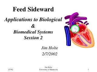
Feed Sideward Applications to Biological & Biomedical Systems Session 2. Jim Holte 2/7/2002. Sessions. Session 1 - Feed Sideward – Concepts and Examples, 1/15 Session 2 – Feed Sideward – Applications to Biological & Biomedical Systems, 2/7

E N D
Feed SidewardApplications to Biological & Biomedical SystemsSession 2 Jim Holte 2/7/2002 Jim Holte University of Minnesota
Sessions • Session 1 - Feed Sideward – Concepts and Examples, 1/15 • Session 2 – Feed Sideward – Applications to Biological & Biomedical Systems, 2/7 • Session 3 – Chronobiology, 2/21 ?Franz Hallberg and Germaine Cornelissen Jim Holte University of Minnesota
Biomedical Devices • Pacemakers - Companies are introducing circadian rhythm based pacemakers. The pacing strategy (amplitude & timing of pacing stimulus) for effective cardiac capture depends on the time of day. (eg. work & sleep). • Drug Delivery - Medtronic/Minimed’s insulin pump has a drug delivery strategy. It is preprogrammed for continuous insulin delivery which depends on exercise, food intake, patient endogenous performance, may now use adjustment of dose as a function of time of day. Jim Holte University of Minnesota
Summary • Dynamical systems analysis provides a technique for designing rate-control biomedical devices for therapeutic diagnosis & intervention. • Rate-control provides direct access to bio-rhythms. • Rate control techniques can apply the extensive knowledge of heart rate variability without requiring knowledge of the causes. • The above builds on the extensive modeling of controllability and extensibility - opaque-box techniques. DS <-> Rate Control <-> bio-rhythm rate variability knowledge <-> opaque-box engineering techniques Jim Holte University of Minnesota
G In Out Σ β G In Out Σ Control G1 In Out G2 Feed Sideward TermsSimple Example • Feed Back Reinvesting dividends • Feed Foreward Setting money aside • Feed Sideward Moving money to another account Jim Holte University of Minnesota
Introduction Feed Sideward is a coupling that shifts resources from one subsystem to another • Feed Sideward #1 – feeds values of other variables into the specified variable • Feed Sideward #2 – feeds changes of parameters into the specified variable. (time varying parameters) • Feed Sideward #3 – feeds changes of topology by switch operations (switched systems) Tool for global analysis especially useful for biological systems Jim Holte University of Minnesota
References • Colin Pittendrigh & VC Bruce, An Oscillator Model for Biological Clocks, in Rhythmic and Synthetic Processes in Growth, Princeton, 1957. • Theodosios Pavlidis, Biological Oscillators: Their mathematical analysis, Princeton, 1973, Chapter 5, Dynamics of Circadian Oscillators • J.D. Murray, Mathematical Biology, Springer-Verlag, 1993, Chapter 8 “Perturbed and Coupled Oscillators …” • Arthur Winfree, The Timing of Biological Clocks, Scientific American Books, 1987 Jim Holte University of Minnesota
Inherent Biological Rhythms • Biosystems Rhythms • second cycles (sec) - cardiac • circadian (day) - sleep cycle) - melatonin (pineal) • circaseptan (week) - mitotic activity of human bone marrow, balneology, bilirubin cycle neonatology • circalunar cycles (month) - menstrual cycle • annual (year) cycles - animal’s coats – weight loss & gain by the season. Jim Holte University of Minnesota
Synchronizers • Exogenous (external) • stimulated by light, temperature & sleep/wake, barometric pressure & headaches/joint aches, • Endogenous (internal): • heart rates • escape beats • preventricular contractions - ectopic beats • Sino-atreal node (associations of myocardial fibers on basis of enervation by vagus nerve) • SA node beats spontaneously, governed by nerve & chemical, SA node stimulates the AV node providing a time delay. • AV node sends excitation through conduction system to the purkinje fibers which stimulate the heart walls to contract. • EEG rhythms (4-30 Hz, alpha, beta, theta & delta) Jim Holte University of Minnesota
Mathematics • Mathematical linkage to synchronizers • Endogenous rhythms refer to the eigenvectors. • Exogenous rhythms refer to the particular integrals (forcing function). dX/dt = AX +B, B provides a forcing function. AX provides the eigenvectors. Jim Holte University of Minnesota
Viewpoint Challenge • Traditional view – biological rhythms are exogenous • Focus on particular integrals (heterogenous eqn, x’=ax+b) • Blood pressure variation is interpreted as an activity variation, thus external. • Now, many claim that biological rhythms are endogenous • Focus on eigenvectors (homogeneous eqn, x’=ax). • Chronobiology viewpoint • Blood pressure variation is interpreted as a hormonal variation, thus internal. Jim Holte University of Minnesota
Nollte Model • Variation of Pavlidis, Eqns 5.4.1 & 5.4.2 • Dynamical System r’=r-cs+b, r>=0 s’=r-as s>=0 r is heart rate, r’ is dr/dt s is blood pressure, s’ is ds/dt b is ambient temperature Jim Holte University of Minnesota
r(0) A half- oscillator r r’ Σ r ∫ b -c -a -cs r’=r-cs+b -as s’=r-as s s’ Σ ∫ B half- oscillator r s(0) r Dynamical System – Circuit Map Jim Holte University of Minnesota
Limit Cycle • r’=r-cs+b, r>=0 • s’=r-as s>=0 • r is heart rate, r’ is dr/dt • s is blood pressure, s’ is ds/dt • b is ambient temperature • a = 0.5, c = 0.6, e = 0.5, ep = 0.1, b = 0.3 • Initial r = 0, s = 25, file = CIRC-CL10.ODX Jim Holte University of Minnesota
Effect of Increased Heart Rate • r’=r-cs+b, r>=0 • s’=r-as s>=0 • r is heart rate, r’ is dr/dt • s is blood pressure, s’ is ds/dt • b is ambient temperature • a = 0.5, c = 0.6, e = 0.5, ep = 0.1, b = 0.3 • Initial r = 36, s = 40, file = CIRC-CL11.ODX Jim Holte University of Minnesota
Effect ofDecreased Heart Rate • r’=r-cs+b, r>=0 • s’=r-as s>=0 • r is heart rate, r’ is dr/dt • s is blood pressure, s’ is ds/dt • b is ambient temperature • a = 0.5, c = 0.6, e = 0.5, ep = 0.1, b = 0.3 • Initial r = 30, s = 40, file = CIRC-CL12.ODX Jim Holte University of Minnesota
Effect of Critical Heart Rate & Pressure • r’=r-cs+b, r>=0 • s’=r-as s>=0 • r is heart rate, r’ is dr/dt • s is blood pressure, s’ is ds/dt • b is ambient temperature • a = 0.5, c = 0.6, e = 0.5, ep = 0.1, b = 0.3 • Initial r = 1.5, s = 3, file = CIRC-CL13.ODX Jim Holte University of Minnesota
Effect of Perturbed Equilibrium • r’=r-cs+b, r>=0 • s’=r-as s>=0 • r is heart rate, r’ is dr/dt • s is blood pressure, s’ is ds/dt • b is ambient temperature • a = 0.5, c = 0.6, e = 0.5, ep = 0.1, b = 0.3 • Initial r = 1.5, s = 2.5, file = CIRC-CL14.ODX Jim Holte University of Minnesota
Biomedical Devices • Pacemakers - Companies are introducing circadian rhythm based pacemakers. The pacing strategy (amplitude & timing of pacing stimulus) for effective cardiac capture depends on the time of day. (eg. work & sleep). • Drug Delivery - Medtronic/Minimed’s insulin pump has a drug delivery strategy. It is preprogrammed for continuous insulin delivery which depends on exercise, food intake, patient endogenous performance, may now use adjustment of dose as a function of time of day. Jim Holte University of Minnesota
Summary • Dynamical systems analysis provides a technique for designing rate-control biomedical devices for therapeutic diagnosis & intervention. • Rate-control provides direct access to bio-rhythms. • Rate control techniques can apply the extensive knowledge of heart rate variability without requiring knowledge of the causes. • The above builds on the extensive modeling of controllability and extensibility - opaque-box techniques. DS <-> Rate Control <-> bio-rhythm rate variability knowledge <-> opaque-box engineering techniques Jim Holte University of Minnesota
Next Session • Session 1 - Feed Sideward – Concepts and Examples, 1/15 • Session 2 – Feed Sideward – Applications to Biological & Biomedical Systems, 2/7 • Session 3 – Chronobiology, 2/21 ?Franz Hallberg and Germaine Cornelissen Jim Holte University of Minnesota
Jim Holte University of Minnesota
Backup Jim Holte University of Minnesota
Solution Source: Pavlidis, p. 109 Jim Holte University of Minnesota
Nollte Model:Continuous Extension y = a + (b-a)*[(x-a1)/(b1-a1)] Jim Holte University of Minnesota
ODE Architect Models Jim Holte University of Minnesota
References • Colin Pittendrigh & VC Bruce, An Oscillator Model for Biological Clocks, in Rhythmic and Synthetic Processes in Growth, Princeton, 1957. • Theodosios Pavlidis, Biological Oscillators: Their mathematical analysis, Princeton, 1973, Chapter 5, Dynamics of Circadian Oscillators • J.D. Murray, Mathematical Biology, Springer-Verlag, 1993, Chapter 8 “Perturbed and Coupled Oscillators …” • Arthur Winfree, “The Temporal Morphology of a Biological Clock”, Amer Math Soc, Lectures on Mathematics in the Life Sciences, Gerstenhaber, 1970, p 111-150 • Arthur Winfree, “Integrated View of Resetting a Circadian Clock, Journ Theoretical Biology, Vol 28, pp 327-374, 1970 • Arthur Winfree, The Timing of Biological Clocks, Scientific American Books, 1987 Jim Holte University of Minnesota
Feed Sideward - Topics (60 min) • Session 2 (12 slides) • Applications to Biological Systems • Circadian & other Rhythms (2 slides) • Model & Simulation Result (2 slides) • Applications to Biomedical Systems • Blood Pressure Application (2 slides) • Model & Simulation Result (2 slides) • Summary (1 slide) • Segue to Chronobiology (1 slide) Session 1 (14 slides) • Background Concepts & Examples • Phase Space (1 slide) • Singularities (2 slides) * • Coupled Oscillators (2 slides) • Phase Resetting (2 slides) * • Oscillator Entrainment (1 slide) • Feed Sideward as modulation (3 slides) ** • Summary (1 slide) Jim Holte University of Minnesota
Feed SidewardUnderstandingBiological RhythmsSession 1 Jim Holte 1/15/2002 Jim Holte University of Minnesota
Sessions • Session 1 - Feed Sideward – Concepts and Examples, 1/15 • Session 2 – Feed Sideward – Applications to Biological & Biomedical Systems, 1/31 • Session 3 – Chronobiology, 2/12Franz Hallberg and Germaine Cornalissen Jim Holte University of Minnesota
G In Out Σ β G In Out Σ Control G1 In Out G2 Feed Sideward TermsSimple Example • Feed Back Reinvesting dividends • Feed Foreward Setting money aside • Feed Sideward Moving money to another account Jim Holte University of Minnesota
Introduction Feed Sideward is a coupling that shifts resources from one subsystem to another • Feed Sideward #1 – feeds values of other variables into the specified variable • Feed Sideward #2 – feeds changes of parameters into the specified variable. (time varying parameters) • Feed Sideward #3 – feeds changes of topology by switch operations (switched systems) Tool for global analysis especially useful for biological systems Jim Holte University of Minnesota
Phase Space • Laws of the physical world • Ordinary differential equations • Visualization of Solutions • Understanding Jim Holte University of Minnesota
H t P P With t markers t H Phase Space The Lotka-Volterra Equations for Predator-Prey Systems H' = b*H - a*H*P P' = -d*P + c*H*P H = prey abundance, P = predator Set the parameters b = 2 growth coefficient of prey d = 1 growth coefficient of predators a = 1 rate of capture of prey per predator per unit time c = 1 rate of "conversion" of prey to predators per unit time per predator. Source: ODE Architect, Wiley, 1999 Jim Holte University of Minnesota
Phase Space The Lotka-Volterra Equations for Predator-Prey Systems H' = b*H - a*H*P P' = -d*P + c*H*P H = prey abundance, P = predator Set the parameters b = 2 growth coefficient of prey d = 1 growth coefficient of predators a = 1 rate of capture of prey per predator per unit time c = 1 rate of "conversion" of prey to predators per unit time per predator. Source: ODE Architect, Wiley, 1999 Jim Holte University of Minnesota
Coupled Oscillators Model • x and y represent the "phases“ of two oscillators. Think of x and y: • angular positions of two "particles" • moving around the unit circle • a1 = 0 • x has constant angular rate • a2 = 0 • y has constant angular rate. • Coupling when a1 or a2 non-zero Source: ODE Architect, Wiley, 1999 Jim Holte University of Minnesota
The Tortoise and the Hare x' = w1 + a1*sin(y - x) y' = w2 + a2*sin(x - y) u = (x mod(2*pi)) //Wrap around the v = (y mod(2*pi)) //unit circle phi = (x - y)mod(2*pi) Set the parameters a1 = 0.0; a2 = 0.0 w1 = pi/2; w2 = pi/3 ExampleUncoupled Oscillators Source: ODE Architect, Wiley, 1999 Jim Holte University of Minnesota
Coupled Oscillators: The Tortoise and the Hare x' = w1 + a1*sin(y - x) y' = w2 + a2*sin(x - y) u = (x mod(2*pi)) //Wrap around the v = (y mod(2*pi)) //unit circle phi = (x - y)mod(2*pi) Set the parameters a1 = 0.5; a2 = 0.5 w1 = pi/2; w2 = pi/3 ExampleCoupled Oscillators Source: ODE Architect, Wiley, 1999 Jim Holte University of Minnesota
+1 PULSE_UP STIM T1 T2 -1 PULSE_DOWN Phase Resetting FUNCTION PULSE_UP(t, T1, STIM_H) IF (t >= T1) THEN PULSE_UP = STIM_H ELSE PULSE_UP = 0 ENDIF RETURN PULSE_UP END FUNCTION STIM(t,T1,T2,STIM_L,STIM_H) STIM = PULSE_UP(t, T1, STIM_H) + PULSE_DOWN(t, T2, STIM_L) RETURN STIM END FUNCTION PULSE_DOWN(t,T2,STIM_L) IF (t <= T2) THEN PULSE_DOWN = 0 ELSE PULSE_DOWN = STIM_L ENDIF RETURN PULSE_DOWN END Jim Holte University of Minnesota
Theta' = 1 + STIM(t,T1,T2,STIM_L,STIM_H)*cos(2*Theta) T1 = 4 T2 = 4 STIM_L = -1 STIM_H = +1 Theta' = 1 + STIM(t,T1,T2,STIM_L,STIM_H)*cos(2*Theta) T1 = 4 T2 = 6 STIM_L = -1 STIM_H = +1 ExamplePhase Resetting Source: ODE Architect, Wiley, 1999 Jim Holte University of Minnesota
Oscillator Entrainment • x and y represent the "phases“ of two oscillators. • Think of x and y: • angular positions of two "particles" • moving around the unit circle • a1 = 0 • x has constant angular rate • a2 = 0 • y has constant angular rate. • Coupling when a1 & a2 non-zero • Entrainment occurs when the coupling causes • angular rate of x to • approach angular rate of y • x and y generally differ • Typical for Chronobiology • Dominant oscillator ‘entrains’ the other Source: ODE Architect, Wiley, 1999 Jim Holte University of Minnesota
Oscillator Entrainment Example x' = w1 + a1*sin(y - x) y' = w2 + a2*sin(x - y) u = (x mod(2*pi)) //Wrap around the v = (y mod(2*pi)) //unit circle phi = (x - y)mod(2*pi) Set the parameters a1 =.0775*pi; a2 =.075*pi w1 = pi/4; w2 = pi/4 - .14*pi Source: ODE Architect, Wiley, 1999 Jim Holte University of Minnesota
Singularities r' = -(r-0)*(r-1/2)*(r-1) - a*STIM(t,T1,T2,STIM_L,STIM_H) theta' = 1 x = r*cos(theta) y = r*sin(theta) T1 = 4 T2 = 6 a=0.0 STIM_L = -1 STIM_H = +1 Jim Holte University of Minnesota
Example - Singularities Run r a Commment --- --- --- --------- #1 1.25 0 approaches r=1 #2 1.0 0 stable periodic orbit #3 0.75 0 approaches r=1 #4 0.5 0 unstable periodic orbit #5 0.25 0 approaches r=0 #6 0 0 stable periodic orbit #7 0.75 0.4 starts in r=1 domain, STIM moves it to r=0 domain r' = -(r-0)*(r-1/2)*(r-1) - a*STIM(t,T1,T2,STIM_L,STIM_H) theta' = 1 x = r*cos(theta) y = r*sin(theta) T1 = 4 T2 = 6 a=0.0 STIM_L = -1 STIM_H = +1 Source: Holte & Nolley, 2002 Jim Holte University of Minnesota
G In Out Σ β G In Out Σ Control G1 In Out G2 Feed Sideward TermsSimple Example • Feed Back Reinvesting dividends • Feed Foreward Setting money aside • Feed Sideward Moving money to another account Jim Holte University of Minnesota
Feed Sideward Example The Oregonator Model for Chemical Oscillations x' = a1*(a3*y - x*y + x*(1-x)) y' = a2*(-a3*y - x*y + f*z) z' = x - z smally = y/150 a1 = 25; a3 = 0.0008; a2 = 2500; f = 1 Source: ODE Architect, Wiley, 1999 Jim Holte University of Minnesota
Summary Feed Sideward is a coupling that shifts resources from one subsystem to another • Feed Sideward #1 – feeds values of other variables into the specified variable • Feed Sideward #2 – feeds changes of parameters into the specified variable. (time varying parameters) • Feed Sideward #3 – feeds changes of topology by switch operations (switched systems) Tool for global analysis especially useful for biological systems Jim Holte University of Minnesota
Next Session • Session 1 - Feed Sideward – Concepts and Examples, 1/15 • Session 2 – Feed Sideward – Applications to Biological & Biomedical Systems, 1/31 • Session 3 – Chronobiology, 2/12Franz Hallberg and Germaine Cornelissen Jim Holte University of Minnesota