Download

1 / 37
370 likes | 480 Vues
This work delves into the concept of emergence in economic systems, emphasizing how macroscopic properties arise from the interactions of microscopic agents. It critiques traditional economic approaches that focus on averages and uniform growth, suggesting instead that exceptional cases and diverse behaviors drive economic outcomes. Drawing on historical data and interdisciplinary theories, it explores how to foster growth in challenging conditions, highlighting the need for new thinking in economics that accommodates complexity and variability.

E N D
Complexity Emergence in Economics Sorin Solomon, Racah Institute of Physics HUJ Israel Scientific Director of Complex Multi-Agent Systems Division, ISI Turin and of the Lagrange Interdisciplinary Laboratory for Excellence In Complexity Coordinator of EU General Integration Action in Complexity ScienceChair of the EU Expert Committee for Complexity Science MORE IS DIFFERENT (Anderson 72; Nobel for Physics 77)(more is more than more)Complex“Macroscopic” properties may be the collective effect of many simple “microscopic” components Phil Anderson “Real world is controlled … • by the exceptional, not the mean; • by the catastrophe, not the steady drip; • by the very rich, not the ‘middle class’. we need to free ourselves from ‘average’ thinking.”
“MORE IS DIFFERENT” Complex Systems Paradigm MICRO - the relevant elementary agents INTER - their basic, simple interactions MACRO - the emerging collective objects Traders, investors transactions herds,crashes,booms Decision making, psychology economics statistical mechanics, physicsmath, game theory, info • Intrinsically (3x) interdisciplinary: • MICRO belongs to one science • MACRO to another science • Mechanisms: a third science
“Levy, Solomon and Levy'sMicroscopic Simulation of Financial Marketspoints us towardsthe future of financial economics” HARRY M. MARKOWITZ, Nobel Laureatein Economics1990
Suppose you are the president of a region, or the president of its industrialists association The new statistics are in: the economy is decaying by 10%. Is it good news or bad news? On top of it , some of the major enterprises (representing 50% of the economy) are decaying by 40%. Is it good news or bad news?
If the average growth rate is -10% and the major enterprises (50% of the economy) are going down by -40%,it means that there are enterprises in the other 50% that are growing by + 20%. If you let them develop, in 4 years: they will grow by (1.20)4 = double ! (they alone will equal the volume of the total initial economy). From that moment on, the region economy will have a total growth rate of ~ 20%
What would be the worse thing to do? To try to insure a uniform rate of growthby differential taxation and subsidies: Put togetherthe -40% of the losers,with the +20% of the successful and get together a uniform NEGATIVE growth rate -10%: everybody collapses!
These scenarios look oversimplified, unrealistic and unpractical but actually this is somewhatwhat happened [in both directions] in quite a number of countries around the 1990’s.
I present in the sequel data and theoretical study of Poland's 3000 counties over 15 years following the 1990 liberalization of the economy. The data tells a very detailed story similar to the above but a little bit more sophisticated. To understand it we have to go back in time more then 200 years ago in Holland. (but don't worry, we will soon get back toTorino (Pareto, Volterra) to get more info).
Malthus : autocatalitic proliferation/ returns :B+AB+B+Adeath/ consumption B Ø dw/dt = awa =(#A x birth rate - death rate)a=(#A x returns rate - consumption /losses rate) exponential solution: w(t) = w(0)e a t w= #B birth rate > death rate a > 0 birth rate > death rate a < 0 TIME
Solution: exponential==========saturation at X= a / c Verhulst way out of it: B+B BThe LOGISTIC EQUATION dw/dt = a w – c w2 c=competition / saturation w = #B
almost all the social phenomena, except in their relatively brief abnormal times obey the logistic growth.“Social dynamics and quantifying of social forces”Elliott W. Montroll US National Academy of Sciences and American Academy of Arts and Sciences 'I would urge that people be introduced to the logistic equation early in their education… Not only in research but also in the everyday world of politics and economics …”Nature Robert McCredie, Lord May of Oxford, President of the Royal Society
SAME SYSTEM Reality Models Discrete Individuals ContinuumDensity Complex ----------------------------------Trivial Localized patches-----------------------Spatial Uniformity Adaptive ----------------------------------Fixed dynamical law Development -----------------------------Decay Survival -----------------------------------Death Misfit was always assigned to the neglect of specific details. We show it was rather due to the neglect of the discreteness.Once taken in account => complex adaptive collective objects. emerge even in the worse conditions
Logistic Equation usually ignored spatial distribution,Introducediscretenessandrandomeness ! w. = ( conditions x birth rate - death) xw+diffusion w - competition w2 conditions is a function ofmany spatio-temporal distributed discrete individual contributionsrather then totally uniform and static
Phil Anderson “Real world is controlled … • by the exceptional, not the mean; • by the catastrophe, not the steady drip; • by the very rich, not the ‘middle class’ we need to free ourselves from ‘average’ thinking.”
Shnerb, Louzoun, Bettelheim, Solomon,[PNAS (2000)] proved by (FT,RG) that the continuum , differential logistic equation prediction: Multi-Agent <a> << 0prediction Differential Eqations(continuum <a> << 0approx) Time Instead: emergence of singularspatio-temporal localizedcollective islands with adaptive self-serving behavior Is ALWAYS wrong ! => resilience and sustainabilityeven for <a> << 0!
Electronic Journal of Probability Vol. 8 (2003) Paper no. 5, pages 1–51. Branching Random Walk with Catalysts Harry Kesten, Vladas Sidoravicius Shnerb et al. (2000), (2001) studied the following system of interacting particles on Zd: There are two kinds of particles, called A-particles and B-particles. The A-particles perform continuous time simple random walks, independently of each other. The jumprate of each A-particle is DA. The B-particles perform continuous time simple random walks with jumprate DB, but in addition they die at rate and a B-particle at x at time s splits into two particles at x during the next ds time units with a probability NA(x, s)ds+o(ds), where NA(x, s) (NB(x, s)) denotes the number of A-particles (respectively B-particles) at x at time s. Conditionally on the A-system, the jumps, deaths and splittings of different B-particles are independent. Thus the B-particles perform a branching random walk, but with a birth rate of new particles which is proportional to the number of A-particles which coincide with the appropriate B-particles. One starts the process with all the NA(x, 0), x 2 Zd, as independent Poisson variables with mean μA, and the NB(x, 0), x 2 Zd, independent of the A-system, translation invariant and with mean μB. Shnerb et al. (2000) made the interesting discovery that in dimension 1 and 2 the expectation E{NB(x, t)} tends to infinity, no matter what the values of , ,DA, DB, μA, μB 2 (0,1) are.
We have only changed the notation slightly and made more explicit assumptions on the initial distributions than Shnerb et al. (2000). Shnerb et al. (2000) indicates that in dimension 1 or 2 the B-particles “survive” for all choices of the parameters , ,DA,DB, μA, μB > 0. However, they deal with some form of continuum limit of the system and we found it difficult to interpret what their claim means for the system described in the abstract. For the purpose of this paper we shall say that the B-particles survive if lim sup t!1 P{NB(0, t) > 0} > 0, (1.1) where P is the annealed probability law, i.e., the law governing the combined system of both types of particles. We shall see that in all dimensions there are choices of , ,DA,DB, μA, μB > 0 for which the B-particles do not survive in the sense of (1.1). A much weaker sense of survival is that lim sup t!1 ENB(0, t) > 0. (1.2) Our first theorem confirms the discovery of Shnerb et al. (2000) that even more than (1.2) holds in dimension 1 or 2 for all positive parameter values. Note that E denotes expectation with respect to P, so that this theorem deals with the annealed expectation. Theorem 1. If d = 1 or 2, then for all , ,DA,DB, μA, μB > 0 ENB(0, t) ! 1 faster than exponentially in t. (1.3) Despite this result, it is not true that (1.1) holds for all , ,DA,DB, μA, μB > 0. In fact our principal result is the following theorem, which deals with the quenched expectation (i.e., in a fixed realization of the catalyst system). Here FA := -field generated by {NA(x, s) : x 2 Zd, s 0}.
w. = a w –c w2 Logistic Diff Eq prediction: Multi-Agent stochastic<a> << 0prediction Differential Equationscontinuum<a><< 0approx) Time GDP Poland Nowak, Rakoci, Solomon, Ya’ari
The GDP rate of Poland, Russia and Ukraine (the 1990 levels equals 100 percent) Poland Russia Ukraine
Belarus Slovakia Kazahstan Hungary
One may represent the dynamics of the counties economies by the following system of coupled differential equations d wi / dt = (ai-∑jrji)wi+ ∑jrij wj– ∑jwi cik wk d wi / dt = the growth rate of county i aiwi=endogenous proliferation rate in county i ∑jrij wj = the growth due to transfer from other counties -∑jrjiwi =the capital transfer to other counties ∑jwi cik wk= the competition and other interaction factors with other counties and the environment
Predicted Scenario: First the singular educated centers WMAX develop while the others WSLOW decay d wMAX / dt ~(aMAX- ∑jrj ;MAX)wMAX >>0 d wSLOW / dt~(aSLOW-∑jrjSLOW)wSLOW <<0 Then, as WMAX>>WSLOW , the transfer becomes relevant and activity spreads from MAX to SLOW and all develop with the same rateaMAX-∑ jrji but preserve large inequality d wSLOW / dt~rSLOW, MAX wMAX =>wSLOW/wMAX~rSLOW MAX / (aMAX-ai)
Couthy Growth= Local Proliferation + transfer from others + saturation d wi / dt = (ai-∑jrji)wi+ ∑jrij wj– ∑jwi cik wk • Case 1: low level of capital redistributionrj , MAX<< (aMAX – aj ) -high income inequalitywi/wMAX ~ riMAX/(aMAX-ai) -outbreaks of instability(e.g. Russia, Ukraine). • Case2: high level of central capital redistribution(as in the previous, socialist regime) rj , MAX>> (aMAX – aj ) - slow growth or even regressing economy (Latvia) but quite - uniform wealth in space and time. • Case 3 :Poland seems - optimal balance : aj , MAX are large enough to insure adaptability and sustainability over a large number of counties yet the • aMAX -∑j rjMAXis still large enough to insure overall growth.
Romania Poland Russia Latvia Ukraine
Very few localized growth centers (occasionally efficient but unequal and unstable) Intermediate Range Uniform distribution (unefficient but stable (decay))
Prediction the economic inequality (Pareto exponent)and the economic instability (index anomalous fluctuations exponent) It is also strongly confirmed (the data we had were from western economies) a b 400 Forbes 400 richest by rank
Measure Changes in aidue to Fiat plant closure With Prof Terna’s group Check alternatives PIEMONTE MAP