• URL: .../publications/courses/ece_8423/lectures/current/lecture_24

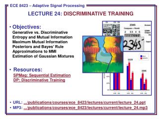
1. LECTURE 24: DISCRIMINATIVE TRAINING • Objectives:Generative vs. DiscriminativeEntropy and Mutual InformationMaximum Mutual InformationPosteriors and Bayes’ RuleApproximations to MMIEstimation of Gaussian Mixtures • Resources:SPMag: Sequential EstimationDP: Discriminative Training • URL: .../publications/courses/ece_8423/lectures/current/lecture_24.ppt • MP3: .../publications/courses/ece_8423/lectures/current/lecture_24.mp3

2. Introduction • There are two types of paradigms for learning statistical classifiers: generative and discriminative models. • Generative models rely on learning the joint probability distribution of the observed features and the corresponding class membership. Class assignments are then made based on assigning the most likely class. The goal is to maximize likelihood thereby indirectly minimizing error rate. • Generative models derive their name from the fact that the model has the ability to synthesize data with the statistical properties similar to the training data. • Techniques we have discussed such as maximum likelihood estimation (MLE) and maximum a posteriori (MAP) estimation fall in this class of algorithms. • Discriminative models directly estimate the class posterior probability. The intermediate step of estimating the joint distribution is bypassed. Class assignments are made based on direct maximization of a discriminant function(s). The goal is to directly minimize error rate. • There are three general classes of discriminative algorithms: maximum mutual information (MMI), minimum classification error (MCE) and minimum “phone” or “word” error (MPE/MWE). We will focus here on MMIE. • New literature is emerging that attempts to describe all three of these approaches from a common framework.

3. Maximum Mutual Information Estimation (MMIE) • MMI classifier design is based on maximizing the mutual information between the observed data and their corresponding labels. • From an information theory perspective, mutual information provides a measure of the amount of information gained, or uncertainty reduced, regarding the labels after seeing the data. • MMI is a well-established principle in information theory and possesses good theoretical properties. • In contrast, the MCE approach uses a classifier that compares a set of discriminant functions. Parameter estimation involves minimizing an expected loss function. Popular techniques such as Support Vector Machines (SVMs) fall in this category. • The MAP/MWE approach is somewhat specific to sequential estimation problems such as speech recognition. Instead of minimizing the overall “sentence” or string of symbols error rate, the approach attempts to optimize performance at the substring level. • All three approaches can be mapped to an objective function in a canonical rational function form in which the denominator term is constrained to be positive valued. • Much of this work dates back to the original work in the late 1960’s by Baum, Dempster and their colleagues.

4. Entropy and Mutual Information • The entropy of a discrete random variable is defined as: • The joint entropy between two random variables, X and Y, is defined as: • The conditional entropy is defined as: • The mutual information between two random variables, X and Y, is defined as: • There is an important direct relation between mutual information and entropy: • By symmetry, it also follows that: • Two other important relations:

5. Mutual Information in Pattern Recognition • Given a sequence of observations, X = {x1, x2, …, xn}, which typically can be viewed as features vectors, we would like to minimize the error in prediction of the corresponding class assignments,  = {1, 2, …,m}. • A reasonable approach would be to minimize the amount of uncertainty about the correct answer. This can be stated in information theoretic terms as minimization of the conditional entropy: • Using our relations from the previous page, we can write: • If our goal is to minimize H(|X), then we can try and minimize H() or maximize I(;X). • The minimization of H() corresponds to finding prior probabilities that minimize entropy, which amounts to accurate prediction of class labels from prior information. (In speech recognition, this is referred to as finding a language model with minimum entropy.) • Alternately, we can estimate parameters of our model that maximize mutual information -- referred to as maximum mutual information estimation (MMIE).

6. Posteriors and Bayes Rule • The decision rule for the minimum error rate classifier selects the class, i, with the maximum posterior probability, P(I |x). • Recalling Bayes Rule: • The evidence, p(x), can be expressed as: • As we have discussed, we can ignore p(x) since it is constant with respect to the maximization (choosing the most probable class). • However, during training, the value of p(x) depends on the parameters of all models and varies as a function of x. • A conditional maximum likelihood estimator, *CMLE, is defined as: • From the previous slide, we can invoke mutual information: • However, we don’t know the joint distribution, p(X,)!

7. Approximations to Mutual Information • We can define the instantaneous mutual information: • If we assume equal priors, then maximizing the conditional likelihood is equivalent to maximizing the instantaneous mutual information. This is referred to as MMIE. • We can expand I(x,i) into two terms, one representing the correct class, and the other representing the incorrect classes (or competing models): • The posterior probability, P(I |x),can be rewritten as: • Maximization of the posterior implies we need to reinforce the correct model and minimize the contribution from the competing models. • We can further rewrite the posterior: implies we must maximize:

8. Additional Comments • This illustrates a fundamental difference: in MLE, only the correct model need be updated during training, while in MMIE, every model is updated. • The greater the prior probability of a competing class label, k, the greater its contribution to the MMIE model, which makes sense since the chance of misrecognizing the input as this class is greater. • Though it might appear MMIE and MLE are related, they will produce different solutions for finite amounts of training data. They should converge in the limit for infinite amounts of training data. • The principal difference is that in MMIE, we decrement the likelihood of the the competing models, while in MLE, we only reinforce the correct model. • MMIE, however, is computationally very expensive and lacks an efficient maximization algorithm. • Instead, we must use gradient descent.

9. Gradient Descent • We will define our optimization problem as a minimization: • No closed-form solution exists so we must use an iterative approach: • We can apply this approach to HMMs. The objective functions used in discriminative training are rational functions. • The original Baum-Welch algorithm requires that the objective function be a homogenous polynomial. • The Extended Baum-Welch (EBW) algorithm was developed for use on rational functions, and applied to continuous density HMM systems. • The reestimation formulas have been derived for the mean and diagonal covariance matrices for a state j and mixture component m:

10. Estimating Probabilities • Mixture coefficients and transition probabilities are a little harder to estimate using discriminative training and have not showed significant improvements in performance. • Similarly, it is possible to integrate mixture splitting into the discriminative training process, but that has provided only marginal gains as well. • There are various strategies for estimating the learning parameter, D, and making this specific to the mixture component and the state. • We note that calculation of the Gaussian occupancies (i.e. the probability of being in state j and component m summed over all time) is required. In MLE training, these quantities are calculated for each training observation using the forward-backward algorithm (and transcriptions of the data). • For MMIE training, we need counts for both the correct model (numerator) and all competing models (denominator). • The latter is extremely expensive and has been the subject of much research. The preferred approach is to use a lattice to approximate the calculation of the probability of the competing models.

11. Summary • Reviewed basic concepts of entropy and mutual information from information theory. • Discussed the use of these concepts in pattern recognition, particularly the goal of minimization of conditional entropy • Demonstrated the relationship between minimization of conditional entropy and mutual information. • Derived a method of training that maximizes mutual information (MMIE). • Discussed its implementation within an HMM framework. • These methods carry the usual concerns about generalization: can models trained on one particular corpus or task transfer to another task? • In practice, generalization has not been robust across widely varying applications or channel conditions. • In controlled environments, performance improvements are statistically significant but not overwhelmingly impressive given the compute requirements. • Next: apply discriminative training to adaptation.