Download
1 / 22
220 likes | 441 Vues
Visualization of vortex states in mesoscopic superconductors. I. Grigorieva, L. Vinnikov, A. Geim (Manchester) V. Oboznov, S. Dubonos (Chernogolovka). Motivation.

E N D
Visualization of vortex states in mesoscopic superconductors I. Grigorieva, L. Vinnikov, A. Geim (Manchester) V. Oboznov, S. Dubonos (Chernogolovka)
Motivation • Vortices in small superconductors (size R ~ξ,λ) expected to behave similar to electrons in artificial atoms, i.e. obey specific rules for shell filling, exhibit magic numbers, etc. • In confined geometries, superconducting wave function must obey boundary conditions which determine total vorticityL • Vortex states are further influenced by vortex interactions with screening currents (for R > λ) • Numerical studies of vortex states exist but so far no direct observations • We present direct observations of vortex states in small superconducting dots by magnetic decoration
Starting Nb films: λ(0) 90 nm; ξ(0) 15 nm; Hc2(0) 1.5 T; 6; Tc=9.1 K; thickness d = 150 nm > ξ, λ Vortex structure in a macroscopic Nb film. External field Hext = 80 Oe
Each structure contained circular disks, squares and triangles of four different sizes: 1µm; 2 µm; 3µm; 5 µm • Over 500 dots decorated in each experiment (same field, temperature, decoration conditions) 200 µm 20 µm 5 µm
experimental details • field-cooling in perpendicular magnetic field • external magnetic field varying between 20 and 160 Oe, i.e., H/Hc2 = 0.002 – 0.016, where Hc2(3.5 K) 1 T; H • decoration captures snapshots of vortex states at T 3.5 K =0.4Tc; • thickness of all nanostructured samples d = 150 nm > ξ, λ
despite strong pinning, confinement has dominating effect on vortex states: • well defined shell structures observed for L 35 in circular disks; • a variety of states with triangular / square symmetries observed for L 15 for triangular and square dots L = 25 (3,8,14) • due to many different combinations of Hext values and dot sizes, almost all possible vorticities between L=0 and L 50 were observed (L = 0,1,2,3,4,5,6,…) • for larger L (L>30-35), vortex arrangements are less well defined and for L > 50 become disordered, similar to macroscopic films L = 9 L = 94
Vorticity vs field • for all values of vorticity L, external filed (total flux) required for nucleation of L vorticies significantly exceeds corresponding field for a macroscopic film
Vorticity vs field experiment, disk size R 100ξ • nucleation of the first vortex requires magnetic flux corresponding to over 30 • states with small vorticities are stable over appreciable field intervals, e.g. for a 2µm disk, H 20 Oe for transition to L=1; H 10 Oe for transition to L=2 B.J. Baelus and F.M. Peeters, Phys. Rev. B 65, 104515, 2002 numerical study, R = 6ξ
Multiplicity of vortex arrangements • at least two or three different states observed in every experiment in dots of nominally the same size 2 m dots, Hext= 80 Oe (3,3,3) (2,7) (2,8) (3,7) (1,8) 3 m dots, Hext= 60 Oe • variations in dot sizes, shape irregularities lead to variations in flux up to 0 • small differences in energy of different states with same L implied (1,8) (3,7) (2,8) (3,3,3) (2,7)
Evolution of vortex states (3,8) (3,7) (2,7) (2,8) (1,8) (1,7) (6) (1,6) (1,5) (5) (4) (3) (2) (1) (0)
Comparison with theory • observed vortex states in good • agreement with numerical • simulations B.J. Baelus, L.R.E. Cabral, F.M. Peeters, Phys.Rev.B 69, 064506 (2004)
Magic numbers • we are able to • identify magic numbers (maximum numbers of vortices in each shell before the next shell nucleates) • identify shell filling rules L = 5 L = 6 … L = 8 L = 7
Magic numbers …after that new vortices appear in either the first or second shell: L=9 (2,7) L=10 (3,7) L=11 (3,8) L=10 (2,8) … and this continues until the total vorticity reaches L=14 (L1=4; L2=10)
Magic numbers … third shell appears at L>14 in the form of one vortex in the centre … L=17 (1,5,11) L=18 (1,6,11) … after that additional vortices nucleate in either first, second or third shell until L3 reaches 16… L=24 (3,7,14) L=22 (2,7,13)
Magic numbers … fourth shell appears at L3>18 in the form of one vortex in the centre, and so on … L=35 (1,5,11,18) • rules of shell filling similar to electrons in artificial atoms (V.M. Bedanov and F.M. Peeters, Phys. Rev.B 49,667, 1994) • magic numbers: one shell L1=6 two shells L2=10 three shells L3=18 …..
Conclusions • direct observations of multiple vortex states in confined geometry • low-vorticity states (L<4) are stable over surprisingly large intervals of magnetic field • well defined shell structures in circular geometry • magic numbers for vortex shell filling
vortex configurations do not change with increasing external field L=20 (1,6,13) Hext=160 Oe L=21 (1,7,13) Hext=160 Oe L=18 (1,6,11) Hext = 30 Oe