Download
1 / 65
660 likes | 690 Vues
Subgrid Scale Fluxes (Land surface, surface layer, PBL and SGS turbulence). Radiation. Comparison with OK Mesonet Measurements. Plots not available. Initial Condition. ARPS Components. Soil Model Initialization. 1 km soil and vegatation data base Soil moisture (and T) Directly from Eta

E N D
Subgrid Scale Fluxes(Land surface, surface layer, PBL and SGS turbulence)
Comparison with OK Mesonet Measurements • Plots not available
Soil Model Initialization • 1 km soil and vegatation data base • Soil moisture (and T) • Directly from Eta • API • 4DVAR retrieval (under development) • Optionally initialization procedure • To reach a balanced initial state
Ways to Initialize ARPS • Idealized, single sounding • Interpolation from GFS, Eta, RUC, etc • ADAS
ARPS Data Analysis System (ADAS) • Manages the real time ingest, QC, objective analysis of observations • Doppler radar data (NIDS, base Level II from n systems, VAD) • MDCRS commercial aircraft wind and temperature reports • Wind profilers • RAOBS (conventional, CLASS, dropsondes) • Mobile and fixed mesonets • SAO and METAR observations • GOES satellite visible and IR data for cloud analysis • NCEP gridded model output • Based on Bratseth successive correction method • Handles retrieved radar data (from SDVR et al) • Had its root in FSL LAPS. Data format is about the only one left though.
Braseth Analysis Scheme • ADAS use the Bratseth analysis scheme which is a successive correction scheme • The scheme theoretically converges to optimal interpolation (O/I), but without explicit inversion of large matrices • Multi-pass strategy used where more detailed data can be introduced after a few iterations using broad-scale data. • Like OI, the Bratseth method accounts for the relative error between the background and each observation source, and is relatively insensitive to large variations in data density. • Vertical correction in terms of z or q
ARPS Data Analysis System (ADAS) • User specifies background error covariances and structure functions. Codes to calculate background error statistics being developed. • Performed on ARPS native (terrain-following) grid • 3-D cloud analysis and diabatic initialization package using GOES, Doppler radar and surface data. • Water vapor, cloud, rain, ice and temperature fields are affected by the cloud analysis • Used to initialize realtime high-res (~kms) forecasts at CAPS since 1996 • Linked closely with ARPS data assimilation system (via, e.g., intermittent assimilation, incremental analysis update method)
Incremental Analysis Update Cycles (from Brewster 2003)
ADAS analysis – Total u ADAS Background 73x73x43 grid, dx=12km
ADAS Analysis– Total q Background ADAS
Example of Initial Condition with cloud analysis on a 3km Grid
ADAS Cloud Analysis Scheme GOES Visible Image at 1745 UTC on 07 May 1995
ADAS Cloud Analysis Scheme Vertical E/W Cross-Section: METAR + GOES IR + WSR-88D
ADAS Cloud Analysis Scheme PW and Vertically Integrated Condensate Valid 13 UTC on 12 April 1999 GOES Visible Image Valid 13 UTC on 12 April 1999
Application to fine-scale analysis at Kennedy Space Center (Case et al 2002 Wea. Forecasting)
ARPS 3DVAR System – Why 3DVAR? Compared to optimal interpolation (OI) or other objective analysis methods, 3DVAR is • Flexible: It can handle data from a variety of sources, including soundings, mesonet, upper air data, satellite, etc., as well as the background; • Powerful. It can perform retrievals (e.g., from satellite radiances and radar reflectivity) at the same time as the analysis by using forward models and their adjoint – i.e., it can make direct use of indirect observations. • For radar data, 3DVAR has the potential to combine the retrievals of single-Doppler velocity and thermodynamic variables, analysis, and initialization into one single step. A good 3DVAR system is an important predecessor to 4D-VAR. • Statistical models, and forward observational operators and their adjoint developed for 3DVAR can be directly used in 4DVAR. • It is less dependent on the prediction model, can therefore be developed before the forward prediction model is completed.
ARPS 3DVAR real wind observed component The Radar Problem: Observe radial velocity and reflectivity only, need V, T, P, qx for IC. For thunderstorms, radar is about the only obs platform! • We describe here a preliminary version of an incremental 3DVAR system developed recently at CAPS • Emphasis is given to the storm-scale and the use of radar data
The ARPS 3DVAR System • The ARPS 3DVAR system will analyze NEXRAD data with or without wind retrievals. • The Jc term, i.e., the dynamic constraints, are currently based on ARPS equations • Incremental formulation
ARPS 3DVAR • Background error covariance initially estimated using the “NMC” method. Flow-dependent covariance estimationmethods will be studied, e.g., that based on ensemble Kalman filter. This is more important for intermittent thunderstorms. • Background covariance is modeled using a simple version of recursive filter. More advanced version will be applied in the future (Purser, et al 2002a,b, Wu et al. 2002) • The analysis vector x contains model primitive variables u, v, w, q, p and q’s,ory (streamfunction), c (velocity potential) , w, q, p and q’s • Coupling among variables and balances are achieved via explicit equation constraints contained in Jc. • Analysis is performed on ARPS native terrain-following grid. • ADAS data handling infrastructure is taken advantage of
Observation Data • Single-level surface data, e.g., • SAO • Mesonet • MDCAR • Multiple-level observations, e.g., • Rawinsondes • Wind profilers • Raw Doppler radial velocity or retrieved velocity fields (via SDVR methods) and reflectivity data
3DVAR Versus ADAS – Total u Background 3DVAR ADAS 73x73x43 grid, dx=12km
3DVAR versus ADAS – Total q Background 3DVAR ADAS
4DVAR and EnKF • 3DVAR lays the foundation for 4DVAR • 3DVAR includes the data handling parts and forward operation operators and their adjoint • Adjoint of an old version of ARPS exists and had been used for cloud scale data assimilation • Adjoint of latest version of ARPS being developed with the help of TAF, an automatic adjoint generator (the commercial version of TAMC) • We are also working on ensemble Kalman filter assimilation
Boundary Conditions • Lateral Boundary Conditions • Rigid, zero-gradient, periodic • Open/radiative LBC (only applied to normal velocity) • Externally (can be from the same model) forced • Davies-type relaxation zone, arbitrary width • w not forced • variables (e.g., water) not found in exbc are excluded from relaxation – zero gradient is usually applied • Ensure same terrain at nesting boundaries • Carpenter (1982) – radiation BC with external forcing(?) • Carpenter, K. M., 1982: Note on radiation conditions for the lateral boundaries of limited-area numerical models. Quart. J. Roy. Meteor. Soc., 108, 717-719.
Vertical Boundary Condition • Radiation top BC based on cosine Fourier transform (Klemp and Durran 1983) • periodicity requirement at the top relaxed • Still based on linearized equations – difficult to apply to large domain • Upper boundary sponge/absorbing layer • relaxation to coarse grid/external model solution in the layer • or relaxation to the mean state • Rigid, zero-gradient and periodic top-bottom BC • Semi-slip lower BC
Two-Way Nesting • Two-way interactive nesting uses the Generalized Adaptive Grid Refinement Interface, a piece of software that I helped Skamarock to develop in the early 1990s • Horizontal nesting only • Allows arbitrary levels and arbitrary number of grids at each level • Allows rotated grids • Allows overlapping grids • Movable via regridding • Quasi-conservative interpolation (quadratic) • Averaged fine grid values replace coarse grid solution • Time interpolation only once every large time step • Used for supercell tornado simulations etc • Terrain issue, MPI
Stratiform Clouds and Precipitation • Microphysics parameterization for grid-scale precipitation • Can be used together with cumulus parameterization schemes • Option to allow condensation at subsatuation (<100% RH) • helps retaining clouds in IC for large grid spacing • improves surface temperature forecast at low-resolution by introducing clouds earlier • Sedimentation term treated implicitly or using time splitting
Microphysics Schemes • Kessler warm rain microphysics (qc and qr) • Lin et al (1983) ice microphysics • includes rain, cloud water, cloud ice, snow, graupel/hail, • lookup tables for power and exponential functions • ice-water saturation adjustment procedure of Tao et al (1989) • modifications to hydrometeo fall speeds (Ferrier 1994 and updated coefficients) • Shultz (1995) simplified ice scheme (also include 3 ice categories)
ARPS Ice Microphysics Processes ~ 30 processes
Accumulated Precipitation from 1977 Del City Supercell Storms with warmrain and ice microphysics
Simulation of 1977 Del City Supercell Storms with warmrain and ice microphysics
Problems • High precipitation biases at high-resolutions with explicit schemes • resolution problem? • fall speed problem? • process problems? • problem with assumed size distributions • High-precip bias with K-F scheme at high-precip threshold • Still, high-resolution (~3km) precipition forecast with explicit scheme is better than coarser (~9km) grids
CAPS Real Time Forecast Domain during IHOP_2002 183×163 273×195 213×131
Convective Clouds and Precipitation • At high resolutions (=< 3km), use ‘explicit’ microphysics, hopefully the model can resolve the convection well • Cumulus parameterization schemes • Kuo scheme • Old and new Kain-Fritch schemes • Betts-Miller-Janjic scheme • New K-F scheme used most