Download
1 / 20
210 likes | 344 Vues
Large-scale hydrometeorology: Integrating land-surface models with observations. By: Ben Livneh. Overview. Background: significance of large-scale land surface modeling Past and ongoing projects Importance of linking models together to capture key land surface processes.

E N D
Large-scale hydrometeorology: Integrating land-surface models with observations By: Ben Livneh
Overview • Background: significance of large-scale land surface modeling • Past and ongoing projects • Importance of linking models together to capture key land surface processes. • The emerging utility of large-scale remote sensing data and the need for improvinggeophysical information transfer • Future directions
Big picture Role of large-scale(several km2 to >105km2) land surface models (LSMs): • Represent the exchanges of energy, water, and carbon at the land surface (affects climate, water availability, ecology, etc…). These can be coupled with atmospheric models, or run offline • Major types of processes/sub-components for the land surface: • Hydrology specific models: surface water budget, soil moisture, stream flow. • Biogeophysical models: vegetation dynamics, crop yield, etc.. • Water quality and sediment transport models • Reservoir model: dams, hydraulic controls • Snow model – including snow, ice, and glaciers • Land surface models (LSMs) may include some, or all of these; represent an integration of many complex processes that are often inter-related. • Linking models is beneficial when one single sub-model /process is not detailed enough. Entails interdisciplinary synergy and promotes learning http://manmadeclimatechange.co.uk/dir./?p=13
Big picture • Models provide a means to estimate conditions over large areas, where detailed observations are not available.Sophisticated methods for transferring geophysical information in and out of the modeling system are vital to maximize physical realism. • Geophysical inputs are needed to drive the models; assumptions about spatial representativeness, interpolation, averaging; • Transferring validated simulations to make predictions over data poor regions (ungauged basins). Even for a “gauged” location, not continuous in space –spatial a transfer scheme is needed Satellite/remote sensing data are an emerging tool for understanding land surface processes. However, as a stand-alone, they are presently inadequate (closure of water and energy budgets); require careful interpretation http://manmadeclimatechange.co.uk/dir./?p=13
Example: linking a LSM with a hydrology model • The Noah LSM isused in most of the National Oceanic and Atmospheric Administration (NOAA) coupled weather and climate models. Its principal role in this settingis to partition net radiation into turbulent surface and ground heat fluxes, which are required to characterize the atmospheric model’s lower boundary. • Historically, the quality and complexity of soil moisture and runoff parameterizations have received less attention than the processes above1,2; • Further, the Noah LSM was run offline to simulate streamflow at theNational Centers for Environmental Prediction (NCEP) and National Weather Service (NWS) and was shown to be less skillful in streamflow prediction compared with more hydrologically based models3. RMSE of modeled streamflow Noah VIC Sac Obs 1. Koster et al., 2000; 2. Bastidas et al., 2006; 3. Bohn et al., 2010
Hydrologic considerations • Hydrologic factors such as soil moisture play an important role in modulating climate4,5, cloud formation6, and surface latent heat fluxes through interaction with evapotranspiration (ET)7 • At very large scales, runoff froman LSM ultimately becomes an input to the oceans, important for modeling of oceanic circulation and climate through salinity levels8,9. • The risk is that poor hydrologic characterization from an LSM could carry-through and produce unrealistic estimates of other important quantities 4. Wang and Kumar, 1998; 5. Mahmood and Hubbard, 2003; 6. Wetzel et al., 1996; 7. Xiu, 2001 ; 8. Verseghy, 1996; 9. Arora, 2001
Hydrologic prediction NWS River Forecast Centers • Long history of Sac usage for flood forecasting/streamflow prediction goes back to 1970s. Hydrologic-based models (e.g. the Sacramento Soil Moisture Accounting model -Sac10) focus on accurately simulating components of the surface water budget, especially streamflow. Sac is used by the NWS River Forecast Centers (RFCs) has been shown to simulate streamflow skillfully compared with other models11. 10. Burnash et al., 1973; 11 Reed et al., 2004 http://water.weather.gov/ahps/rfc/rfc.php
Sac – limitations T P ↑Ecanopy interception through- fall ↑Esoil ↑T infiltration Despite extensive focus on streamflow prediction, 2 notable obstacles prevent Sac from being coupled with atmospheric models or estimate other states and fluxes 1. Lack of a surface energy budget radiative partitioning (downward solar, longwave) surface heat fluxes (sensible, latent) 2. Absence of an explicit vegetation scheme. Affects surface exchanges of heat, moisture and momentum12,13,14 Controls the rate of moisture movement to and from the soil, via canopy interception, root-water uptake T rates shown to vary by vegetation type15 On global average, roughly 2/3 of precip. reaching the land surface is estimated returned to the atmosphere via ET!16 12. Bonan et al., 1992; 13. Pan and Mahrt, 1987; 14; Pielke et al., 1998; 15. Zhang et al., 2001; 16. Tateishi and Ahn
Unified Land Model (ULM) Development • Objective: combine aspects of the soil moisture accounting scheme of the Sacramento model with the versatility of the Noah LSM to create a unified land model (ULM17) capable of representing land surface processes more realistically than either of the existing models. • Assess model performance in estimating important components of the terrestrial water budget ULM SAC model Noah LSM 17. Livneh et al., 2011
Results: evolution of soil moisture and surface heat fluxes through warm season (CA) • Non-linearity of SM decline through dry summer captured only by ULM: dominated first by direct soil evaporation, then transpiration, whereas Noah combines ET sources in Richard’s equation. • ULM surface heat fluxes (not shown) compare favorably with Noah and observations. Important benchmark for model focused on land-atmosphere interaction. Noah ULM Observations
Study domain for further testing and development with remote sensing data, precipitation and streamflow CB MO UM GL GB OH CO AR LM CA EA RG & GU Precipitation stations 13 major hydrologic regions Shaded areas defined by USGS gauge (*suitable scale for comparison with large-scale remote sensing products) 250 MOPEX basins with adequate precipitation gauge density18 18. Schaake et al., 2006
Estimate soil water and snow (TWSC) on the land surface via changes in the Earth’s gravitational field. Gravity Recovery and Climate Experiment (GRACE) Study domain Multi-criteria calibration data Q TWSC Streamflow gages http://www.cosmosmagazine.com/features/online/1678/gravity-ball Estimate ET from the land surface by closing an atmospheric water balance(AWB). Uses gauge precipitation data and North American Regional reanalysis (NARR). Estimate ET from satellite data – differences in vegetation diversity and surface skin temperature ETSAT ETAWB
Single and multi-criteria results19 California Arkansas Red • At large-scales (>105 km2), high-quality single criterion calibrations (TWSC, ET, Q) were tenable. • Multi-criteria calibrations considering Q performed best, while ET and/or TWSC alone did not contain enough information to significantly improve Q simulation. Missouri Colorado Columbia Upper Miss. Ohio multi-criteria calibrations At catchment scales (102 – 104 km2), the best Q predictions resulted from simultaneous calibration towards Q and ETsatellite for 1/3 of cases (80 basins), demonstrating the potential for remote sensing in LSM development Nash-Sutcliffe Efficiency (NSE) ideal NSE (-∞,1) NSE = 1 Perfect model; NSE = 0 Equivalent to climatology TWSC ET Q 19. Livneh et al., 2012a
Parameter transfer/regionalization • Motivated towards extending rigorous calibration effort to new domains. • In general, domain-specific model calibration either impossible (due to lack of data), or infeasible (e.g. University of Washington global drought monitor), thus a broadly applicable method was employed. • Procedure – derive predictive relationships between catchment attribute data (meteorological, geomorphic, land-cover, remote-sensing, other databases) and calibrated model parameters. • A large number of candidate catchment attributes available, therefore, a step-wise principal components analysis (PCA) procedure20was selected to maximize their explanatory skill and minimize potential redundancy. 20. Garen, 1990
Regionalization experiment example • Relate calibrated model parameter to spatially varying catchment attributes. • Could be applied to other physical features, model parameters, or processes. “free” “tension” http://www.terragis.bees.unsw.edu.au/terraGIS_soil/sp_water-soil_moisture_classification.html 1 of 388 attributes considered Tension water model parameter % clay (average)
Parameter transfer results • Used a jack-knifing approach – i.e. only information from other basins used to predict parameters for target basin • An additional (global) experiment reduced the catchment attributes to only those that are globally available. 220 Basins LOCAL-ZONAL Local basin NSE Mean NSE 0.54 ULM calibrated 0.44 ULM regionalized 0.41 ULM regionalized global ULM regionalized global Rank • Modest loss of skill for the regionalized model • The approach worked comparatively well for the global case [show mean NSE scores, sequence the plot above]
Opportunities for linking models • Improving vegetation representation/dynamics to better understand implications of global change on the biosphere. • A comparison of several state-of-the-art LSMs revealed considerable disagreement in their ET partitioning (between transpiration, canopy, and soil evaporation) • Alternatively, models can be run as a multi-model ensemble. This is a good way to ‘bracket’ a solution; collaborate; learn about different ways to parameterize a processes. • Multi-model streamflow forecasting project 21 demonstrated the ability of LSMs to make skillful streamflow forecasts at seasonal leads, with only knowledge of soil moisture and snow states • Model intercomparison projects: snow model intercomparison in the Colorado headwaters (snowpack a vital water resource for montane regions) 21. Koster et al., 2000
Opportunities for transferring/inferring geophysical features • Current strategy of transferring model parameters through land surface attributes, statistics could be extended globally and to other physical phenomena. • Geophysical features can be inferred/derived through physical relationships • Ongoing global project22 testing algorithms that estimate down-welling radiation and humidity (infrequently observed) via inputs of only daily temprature and precipitation (more frequently observed) • Related work23 (nearly complete) to make publicly available a 96 year dataset (1915-2010) of sub-daily hydrometeorological fluxes over the U.S. at approximately 6km resolution. • Can incorporate a combination of inference and transfer. 22. Bohn et al., 2012; 23. Livneh et al., 2012b
Future directions • Continue developing/linking models to address scientific problems; global change; flood forecasting, infrastructure loadings. • Driver for collaboration, interdisciplinary synergy and building a diverse research environment • Further explore ways at incorporating emerging observational data into land-surface modeling • Bristol is an ideal place for this, given the diversity of its faculty, high quality facilities, and encouragement towards inter-departmental and international collaboration.