Spatial Interpolation

1. Spatial Interpolation Chapter 13

2. Introduction • Land surface in Chapter 13 • Also a non-existing surface, but visualized as a surface • Statistical surface: precipitation, snow accumulation, water table, population density. • No regular grid pattern available, so interpolation between the points is used

3. Introduction • Spatial interpolation is a process of using points with known values to estimate values at other points. • If mapping precipitation, for example, and there is no weather reporting station within the grid cell, an estimate is based on nearby weather stations. • Spatial interpolation is a means of converting point data into surface data.

4. Introduction • Global and local methods. • Global method uses every control point available to make the estimate of the unknown value. • Local method uses a sample of control points for estimation.

5. Control Points • Control points are points with known values. • Basic assumption in spatial interpolation is that the value to be estimated at a point is more influenced by nearby control points than those that are farther away. • Ideal is well distributed, but uncommon in real world.

6. Global Methods • Trend Surface Analysis approximates points with know values with a polynomial equation. • Trend surface model is a linear or first-order trend surface (least complex) • zxy=b0+b1x+b2y • b is a coefficient based on control points. • least squares fit • Cubic or 3rd order includes hills and valleys

7. Regression Models • Regression model relates a dependent variable to a number of independent variables in an equation which can then be used for prediction or estimation. • Non-spatial models should not be used

8. Global Methods in ARC/INFO and ArcView • ARC/INFO • TREND from 1st to 12th order • REGRESSION (but does not offer model-selection) • ArcView • no menu method • Avenue script (see Box 13.3 in text)

9. Local Methods • Local interpolation method uses a sample of control points in estimating the unknown value. • Proper selection of control points is important. • Package may suggest number of points. • Distribution is more important than number, but more points imply better interpolations

10. Local Methods • Control point selection • Simple option is nearest points • Within a radius • Quadrant/octant

11. Thiessen Polygons • Thiessen polygons are constructed around a sample of known points so that any point within a Thiessen polygon is closer to the polygon’s known point than any other known points. • Delaunay triangulation (same as TIN) • Perpendiculars to each side and midpoint. • Also called Voronoi polygons

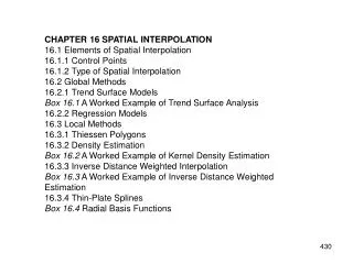
12. Density Estimation • Density estimation measures densities in a grid based on a distribution of their known values. • Simple density: place grid on point distribution and tabulate points that fall within each cell, sum the point values, and estimate density by dividing the total point value by the cell size.

13. Density Estimation • Density estimation measures densities in a grid based on a distribution of their known values. • Kernel estimation: associates each point with kernel function “bump” over bandwidth. • Probability declines farther away from point.

14. Inverse Distance Weighted Interpolation • Inverse distance weighted interpolation method is a local method that assumes that the unknown value of a point is influenced more by nearby control points than those farther away. • Most commonly used in GIS • Degree of influence, or weight, is expressed by the inverse of the distance raised to a power. 1=linear, 2=high near and then declines. • New word of the day! Isohyet (isoline of precipitation)

15. Thin-plate Splines • Thin-plate splines create a surface that passes through the control points and has the least possible change in slope at all points. • steep gradients with data-poor areas. • methods to improve include: thin-plate splines with tension, regularized splines, and regularized splines with tension.

16. Kriging • Kriging is a geo-statistical method for spatial interpolation. • Assumes spatial variation is neither totally random nor deterministic. • Three components: • a spatially correlated component representing the variation of a regionalized variable • a “drift” or structure, representing a trend • a random error term

17. Kriging • Presence or absence of a drift and the interpretation of the regionalized variable have led to development of different kriging methods. • Ordinary kriging: assumes absence of drift, focuses on spatially correlated component • Universal kriging assumes that the spatial variation in z values has a drift or variation in addition to the spatial correlation. • Other: block kriging, co-kriging.

18. Comparison of Local Methods • Similar results, but large errors in data-poor areas • Accuracy must be determined by cross-validation analysis. • remove a point and recalculate comparing the error between estimate and known • if sufficient points, split sample and compare known with estimates • Art or science?

19. Local methods with ARC/INFO and ArcView • ARC/INFO • THIESSEN • POINTDENSITY • IDW • SPLINE • KRIGING • may change in new Geo-statistical Analyst

20. Local methods with ARC/INFO and ArcView • ArcView • Spatial Analyst: density estimation, inverse distance weighted interpolation, and splines (with tension and regularized) • Avenue scripts for kriging