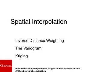
Spatial Interpolation III
Spatial Interpolation III. ENVE 424/524. Spatial Interpolation. We can estimate the value of a variable at a location based on the values of that variable at neighboring locations. The trick is defining the weight. spatial estimation method. z i is the estimated value at location i

Spatial Interpolation III
E N D
Presentation Transcript
Spatial Interpolation III ENVE 424/524
Spatial Interpolation We can estimate the value of a variable at a location based on the values of that variable at neighboring locations. The trick is defining the weight spatial estimation method zi is the estimated value at location i n is the number of data points zj is the value at data point j wij is the weight assigned to data point j continuous surface of estimates (map) point monitoring data
Kriging Steps • Describe the spatial variation in the sample data • Summarize the spatial variation by a mathematical function • Use this model to determine the interpolation weights
Variations on Kriging Simple Uses a known (at least assumed), constant mean across domain. Usually used by subtracting point data values from mean, interpolating the residuals, and then adding back to mean. Universal (kriging with a trend) Uses a modeled trend across domain. The trend is subtracted from the point data values and the residuals interpolated. Indicator kriging Point data are transformed to indicator variables (usually binary). For example, a threshold value is defined and data points that are below the threshold are assigned a value of 1 and those above the threshold are assigned a value of 0. The indicator values are interpolated and the resulting surface shows the probabilities (0-1) of exceeding (or being below) the threshold. Probability Similar to indicator kriging but also incorporates the difference between a data pint value and the defined threshold. Using this “proximity” to threshold information can result in more accurate probabilities.
Block Kriging Used when estimates are required not at points but an average value is required within a prescribed local area. The estimate from block kriging using four points (Figure a) is equal to averaging the estimates from kriging at each of the four points individually.
Kriging with secondary information Kriging can incorporate secondary information to aid the estimation process when the primary variable is sparsely sampled. Secondary information that is physically related to the primary variable and measured at a high spatial density than the primary variable can aid in “filling in” spatial gaps during interpolation. (hard information) (soft information) Examples: Primary Secondary rainfall amount digital elevation model particulate matter concentrations visibility measurements cadmium concentrations zinc concentrations seasonal rainfall (1970-1980) seasonal rainfall (1990-2000)
Kriging with an external drift (KED) A secondary variable related to the primary variable can be used to model the "drift", or trend, of the primary variable in the kriging estimation. In areas without primary sampling sites, the secondary variable aids the estimate through a function relating the secondary to primary variable. As the estimation location gets farther from available primary samples, the estimate approaches the drift value. The secondary variable must vary smoothly in space and must be known at all estimation locations as well as all primary sampling locations. The function relating the secondary and primary variable must be linear. & Ozone measurements in Paris Air quality model grid Ozone concentrations using KED
Cokriging Cokriging is an extension of ordinary kriging that uses a high spatial resolution secondary variable network to improve the estimation of the primary variable. Like ordinary kriging, a variogram model is developed for the primary variable. A second variogram model is developed for the secondary variable A third variogram model is generated from the cross correlation of the primary and secondary variables. The secondary data is "transformed" to the scale of the primary variable in order to derive a cross variogram. The secondary data are then treated identically to the primary data during spatial estimation. All U and V points are paired, binned, and semi-variance calculated U = Secondary Data V = Primary Data V Variogram UV Cross-Variogram U Variogram
Cokriging Example Cokriging does not improve estimates much if -- all the variogram models are very similar in shape -- the secondary information is does not have a higher density than the primary information
Kriging Error Factors influencing interpolation error: • Number of nearby samples • Proximity of nearby samples • Spatial arrangement of samples • Nature of phenomenon being estimated
Cross Validation Cross Validation, a “jackknife technique”, provides a measure of interpolation error Remove site from network (red circle) Obtain estimate at removed site location. Interpolation Error = Estimated Value – Measured Value
Updates ArcGIS now available for class use on the computer in Urbauer 319A Plan is to have it available on two other machines in Cupples II first floor. Reading forerror and uncertainty lectures Focus on Chapters 6 and 15 in Geographic Information Systems and Science, Longley et. Al Optional: Chapter 9 in Principles of Geographical Information Systems, Burrough and McDonnell
Review for Exam Exam will cover material from lecture 1 through today’s lecture Exam questions will be based on problem sets, lecture slides, lab exercises, and the reading. The exam questions will be a mix of: -- multiple choice -- match -- short answer -- equation-based calculations
Types of Attributes A common approach to classifying attributes is based on their level of measurement • Nominal– Simply identifies or labels an entity so that it can be distinguished from another. e.g. sensor ID, building name (Lopata House vs. Lopata Hall) • Cannot be manipulated using mathematical operations. However, frequency distributions are meaningful. • Ordinal – Values based on an order or ranking, e.g. agricultural potential classes • Cannot be manipulated using mathematical operations. However, frequency distributions are meaningful. • Interval – Differences between entities are defined using fixed equal units, e.g. Celsius temperature • Can be manipulated using addition and subtraction • Ratio - Differences between entities can be defined using ratios, e.g. distance • Can be manipulated using multiplication and division • Cyclic - differences between entities depend on direction, e.g. wind direction