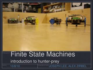
Finite State Machines

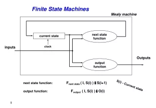
Finite State Machines Chapter 5

Languages and Machines

Regular Languages Generates Regular Language Regular Grammar Recognizes or Accepts Finite State Machine

Finite State Machines An example FSM: a device to solve a problem (dispense drinks); or a device to recognize a language (the “enough money” language that consists of the set of strings, such as NDD, that drive the machine to an accepting state in which a drink can be dispensed) N: nickle D: dime Q: quarter S: soda R: return Accepts up to $.45; $.25 per drink After a finite sequence of inputs, the controller will be in either: A dispensing state (enough money); or a nondispensing state (no enough money) Error!

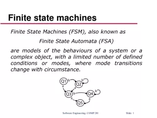
Representations • State diagrams can be used to graphically represent finite state machines. • describe behavior of systems • introduced by Taylor Booth in his 1967 book "Sequential Machines and Automata Theory " • Another representation is the state transition table

FSM • A computational device whose input is a string, and whose output is one of the two values: Accept and Reject • Also called FSA (finite state automata) • Input string w is fed to M (an FSM) one symbol at a time, left to right • Each time it receives a symbol, M considers its current state and the new symbol and chooses a next state • One or more states maybe marked as accepting states • Other stats are rejecting states • If M runs out of input and is in an accepting state, it accepts • Begin defining the class of FSMs whose behavior is deterministic. • move is determined by current state and the next input character

Definition of a DFSM M = (K, , , s, A), where: K is a finite set of states  is an alphabet sK is the initial state AK is the set of accepting states, and  is the transition function from (K) to K

Configurations of DFSMs A configuration of a DFSM M is an element of: K* It captures the two things that can make a difference to M’s future behavior: • its current state • the input that is still left to read The initial configuration of a DFSM M, on input w, is: (s, w)

The Yields Relations The yields-in-one-step relation |-M (q, w) |-M (q', w') iff • w = aw' for some symbol a, and •  (q, a) = q' The relation yields, |-M * , is the reflexive, transitive closure of |-M If Ci |-M * Cj, iff M can go from Ci to Cj in zero (due to “reflexive”) or more (due to “transitive”) steps. Notation: |- and |- * are also used.

Path • A path by M is a maximal sequence of configurations C0, C1, C2 … such that: • • C0 is an initial configuration, • • C0 |-MC1 |-MC2 |-M … • In other words, a path is just a sequence of steps from the start configuration going as far as possible • A path ends when it enters an accepting configuration, or it has no where to go (no transition defined for Cn) • This definition of path is applicable to all machines (FSM, PDA, TM, deterministic or nondeterministic). • A path P can be infinite. For FSM, DPDA, or NDFSM and NDPDA without -transitions, P always ends. For NDFSM and NDPDA with -transitions, P can be infinite. For TM (deterministic or nondeterministic), P can be infinite. • For deterministic machines, there is only one path (ends or not). • A path accepts w if it ends at an accepting configuration • Accepting configuration varies for different machines • A path rejects w if it ends at a non-accepting configuration

Accepting and Rejecting • A DFSM Maccepts a string w iff the path accepts it. • i.e., (s, w) |-M * (q, ), for some qA. • For DFSM, (q, )where qA is an accepting configuration • A DFSM Mrejects a string w iff the path rejects it. • The path, because there is only one. • The language accepted byM, denoted L(M), is the set of all strings accepted by M. • Theorem: Every DFSM M, on input w, halts in at most |w| steps.

Accepting Example • An FSM to accept odd integers: • even odd • even • q0q1 • odd • On input 235, the configurations are: • (q0, 235) |-M (q0, 35) • |-M • |-M • Thus (q0, 235) |-M* (q1, ) • If M is a DFSM and L(M), what simple property must be true of M? • The start state of M must be an accepting state

Regular Languages A language is regular iff it is accepted by some FSM.

A Very Simple Example L = {w {a, b}* : every a is immediately followed by a b}.

Parity Checking L = {w {0, 1}* : w has odd parity}. A binary string has odd parity iff the number of 1’s is odd

No More Than One b L = {w {a, b}* : w contains no more than one b}. Some rejecting states are ignored for clarity

Checking Consecutive Characters L = {w {a, b}* : no two consecutive characters are the same}.

Controlling a Soccer-Playing Robot

A Simple Controller

Programming FSMs L is infinite but M has a finite number of states, strings must cluster: Cluster strings that share a “future”. Let L = {w {a, b}* : w contains an even number of a’s and an odd number of b’s}

Vowels in Alphabetical Order L = {w {a - z}* : can find five vowels, a, e, i, o, and u, that occur in w in alphabetical order}. abstemious, facetious, sacrilegious

Programming FSMs L = {w {a, b}* : w does not contain the substring aab}. Start with a machine for L: How must it be changed? Caution: in this example, all possible states and transitions are specified. In other examples, if we want to use the trick, need to specify all states and transitions first.

FSMs Predate Computers Some pics by me: 1 2 3 The Prague Orloj, originally built in 1410.

The Abacus

The Jacquard Loom Invented in 1801.

The Missing Letter Language • Let  = {a, b, c, d}. • Let LMissing= • {w : there is a symbol ai not appearing in w}. • Try to make a DFSM for LMissing • Doable, but complicated. Consider the number of accepting states • all missing (1) • 3 missing (4) • 2 missing (6) • 1 missing (4)

Nondeterministic Finite Automata • In the theory of computation, a nondeterministic finite state machine or nondeterministic finite automaton (NFA) is a finite state machine where for each pair of state and input symbol there may be several possible next states. • This distinguishes it from the deterministic finite automaton (DFA), where the next possible state is uniquely determined. • Although the DFA and NFA have distinct definitions, it may be shown in the formal theory that they are equivalent, in that, for any given NFA, one may construct an equivalent DFA, and vice-versa • Both types of automata recognize only regular languages. • Nondeterministic machines are a key concept in computational complexity theory, particularly with the description of complexity classes P and NP. • Introduced by Michael O. Rabin and Dana Scott in 1959 • also showed equivalence to deterministic automata • co-winners of Turing award, citation: • For their joint paper "Finite Automata and Their Decision Problem," which introduced the idea of nondeterministic machines, which has proved to be an enormously valuable concept. Their (Scott & Rabin) classic paper has been a continuous source of inspiration for subsequent work in this field.

Nondeterministic Finite Automata • Michael O. Rabin (1931 - ) • son of a rabbi, PhD Princeton • currently Harvard • contributed in Cryptograph • Dana Stewart Scott (1932 - ) • PhD Princeton (Alonzo Church) • retired from Berkley

Definition of an NDFSM • M = (K, , , s, A), where: • K is a finite set of states •  is an alphabet • sK is the initial state • AK is the set of accepting states, and  is the transition relation. It is a finite subset of • (K ( {})) K

NDFSM and DFSM  is the transition relation. It is a finite subset of • (K ( {})) K • Recall the definition of DFSM: • M = (K, , , s, A), where: • K is a finite set of states •  is an alphabet • sK is the initial state • AK is the set of accepting states, and •  is the transition function from (K) to K

NDFSM and DFSM :(K ( {})) K :(K) to K Key difference: • In every configuration, a DFSM can make exactly one move; this is not true for NDFSM • M may enter a config. from which two or more competing moves are possible. This is due to (1) -transition (2) relation, not function

Sources of Nondeterminism • Nondeterminism is a generalization of determinism • Every DFA is automatically an NDDFA • Can be viewed as a kind of parallel computation • Multiple independent threads run concurrently

Envisioning the operation of M • • Explore a search tree (depth-first): • Each node corresponds to a configuration of M • Each path from the root corresponds to the path we have defined • Alternatively, imagine following all paths through M in parallel (breath-first): • Explain later in “Analyzing Nondeterministic FSMs”

Accepting • Recall: a path is a maximal sequence of steps from the start configuration. • M accepts a string w iff there exists some path that accepts it. • Same as DFSM, (q, ) where qA is an accepting configuration • M halts upon acceptance. • Other paths may: • ● Read all the input and halt in a nonaccepting state, • ● Reach a dead end where no more input can be read. • ● Loop forever and never finish reading the input • The language accepted by M, denoted L(M), is the set of all strings accepted by M. • M rejects a string w iff all paths reject it. • It is possible that, on input w L(M), M neither accepts nor rejects. In that case, no path accepts and some path does not reject.

Optional Initial a L = {w {a, b}* : w is made up of an optional a followed by aa followed by zero or more b’s}.

Two Different Sublanguages L = {w {a, b}* : w = aba or |w| is even}.

Why NDFSM? • High level tool for describing complex systems • Can be used as the basis for constructing efficient practical DFSMs • Build a simple NDFSM • Convert it to an equivalent DFSM • Minimize the result

The Missing Letter Language Let  = {a, b, c, d}. Let LMissing= {w : there is a symbol ai not appearing in w}

Pattern Matching L = {w {a, b, c}* : x, y {a, b, c}* (w = xabcabby)}. A DFSM: Works, but complex to design, error prone

Pattern Matching L = {w {a, b, c}* : x, y {a, b, c}* (w = xabcabby)}. An NDFSM: Why it’s an NDFSM? Why it’s hard to create a DFSM? Nondeterminism: “lucky guesses”

Multiple Keywords L = {w {a, b}* : x, y {a, b}* ((w = xabbaay)  (w = xbabay))}.

Checking from the End L = {w {a, b}* : the fourth to the last character is a}

Analyzing Nondeterministic FSMs Given an NDFSM M, how can we analyze it to determine if it accepts a given string? Two approaches: • Depth-first explore a search tree: • Follow all paths in parallel (breath-first)

Following All Paths in Parallel Multiple keywords: L = {w {a, b}* : x, y {a, b}* ((w = xabbaay)  (w = xbabay))}. For abb: a: {q0, q1} -> b: {q0, q2, q6} -> b: {q0, q3, q6}

Dealing with -transitions eps(q) = {pK : (q, w) |-*M (p, w)}. q: is some state in M eps(q): the set of states of M that are reachable from q by following zero or more -transitions eps(q) is the closure of {q} under the relation {(p, r) : there is a transition (p, , r) }. How shall we compute eps(q)?

An Algorithm to Compute eps(q) eps(q: state) = result = {q}. While there exists some presult and some rresult and some transition (p, , r)  do: Insert r into result. Return result.

An Example of eps eps(q0) = {q0, q1, q2} eps(q1) = {q0, q1, q2} eps(q2) = {q0, q1, q2} eps(q3) = {q3}

Simulating an NDFSM ndfsmsimulate(M: NDFSM, w: string) = • current-state = eps(s). • While any input symbols in w remain to be read do: • c = get-next-symbol(w). • next-state = . • For each state q in current-state do: For each state p such that (q, c, p)  do: next-state = next-stateeps(p). • current-state = next-state. • If current-state contains any states in A, accept. Else reject.

Nondeterministic and Deterministic FSMs • Clearly: {Languages accepted by a DFSM}  • {Languages accepted by an NDFSM} • Theorem: • For each DFSM M, there is an equivalent NDFSM M’. • L(M’ ) = L(M) • More interestingly: • Theorem: • For each NDFSM, there is an equivalent DFSM.

Nondeterministic and Deterministic FSMs Theorem: For each NDFSM, there is an equivalent DFSM. Proof: By construction: Given an NDFSM M = (K, , , s, A), we construct M' = (K', , ', s', A'), where K' = P(K) s' = eps(s) A' = {QK : QA} '(Q, a) = {eps(p): pK and (q, a, p)  for some qQ}

Finite State Machines