Pseudo Random Numbers

1. Pseudo Random Numbers • Random numbers generated by a computer are not really random • They just behave like random numbers • For a large enough sample, the generated values will pass all tests for a uniform distribution • If you look at a histogram of a large number, it will look uniform • Pass chi-square test • Pass Kolmogorov-Smirnov Test • The stream of random numbers will pass all the tests for randomness • Runs test • Autocorrelation test

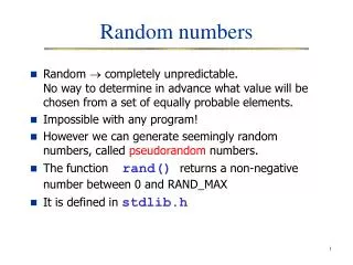
2. Linear Congruential Generators (LCGs) • The most common of several different methods • Generate a sequence of integers Z1, Z2, Z3, … via the recursion Zi = (a Zi–1 + c) (mod m) • a, c, and m are carefully chosen constants • Specify a seed, Z0 to start off • “mod m” means take the remainder of dividing by m as the next Zi • All the Zi’s are between 0 and m – 1 • Return the ith “random number” as Ui = Zi / m

3. Efficient code LCG • LCG with: m = 231 – 1 = 2,147,483,647 a = 75 = 16,807 c = 0 • Cycle length = m – 1

4. Generating Random Variates • Have: Desired input distribution for model (fitted or specified in some way), and RNG (UNIF (0, 1)) • Want: Transform UNIF (0, 1) random numbers into “draws” from the desired input distribution • Method: Mathematical transformations of random numbers to “deform” them to the desired distribution • Specific transform depends on desired distribution • Details in online Help about methods for all distributions • Do discrete, continuous distributions separately

5. Generating from Discrete Distributions • Example: probability mass function • Divide [0, 1] into subintervals of length 0.1, 0.5, 0.4; generate U ~ UNIF (0, 1); see which subinterval it’s in; return X = corresponding value –2 0 3

6. Generating from Continuous Distributions • Example: EXPO (5) distribution Density (PDF) Distribution (CDF) • General algorithm (can be rigorously justified): 1. Generate a random number U ~ UNIF(0, 1) 2. Set U = F(X) and solve for X = F–1(U) • Solving for X may or may not be simple • Sometimes use numerical approximation to “solve”

7. Generating from Continuous Distributions (cont’d.) • Solution for EXPO (5) case: Set U = F(X) = 1 – e–X/5 e–X/5 = 1 – U –X/5 = ln (1 – U) X = – 5 ln (1 – U) • Picture (inverting the CDF, as in discrete case): Intuition: More U’s will hit F(x) where it’s steep This is where the density f(x) is tallest, and we want a denser distribution of X’s

8. Eyeballing • One way to see if a sample of data fits a distribution is to • draw a frequency histogram • estimate the parameters of the possible distribution • draw the probability density function • see if the two shapes are similar frequency data values

9. Chi-Squared Test • Formalizes this notion of distribution fit • Oi represents the number of observed data values in the i-th interval. • pi is the probability of a data value falling in the i-th interval under the hypothesized distribution. • So we would expect to observe Ei = npi, if we have n observations frequency data values pdf data values

10. Chi-Squared Test • So the chi-squared statistic is • By assuming that the Oi - Eiterms are normally distributed, • it can be shown that the distribution of the statistic is approximately chi-squared with k-s-1 degrees of freedom • s is the number of parameters of the distribution • Hint: consider

11. Chi-Squared Test • So the hypotheses are • H0: the random variable, X, conforms to the distributional assumption with parameters given by the parameter estimates. • H1: the random variable does not conform. • The critical value is then • Reject if • This gives a test with significance level .

12. Chi-Squared Test • If the expected frequencies Ei are too small, then the test statistic will not reflect the departure of the observed from the expected frequencies. • The test can reject because of noise • In practice a minimum of Ei 5 is used • If Ei is too small for a given interval, then adjacent intervals can be combined • For discrete distributions • each possible discrete value can be a class interval • combine adjacent values if the Ei’s are too small

13. Chi-Squared Test • For continuous data • intervals that give equal probabilities should be used, not equal length intervals • this gives a better power for the test • the power of test is the probability of rejecting a false hypothesis • it is not known what probability gives the highest power, but we want

14. Kolomogorov-Smirnov Test • Formalizes the idea • The scales are changed by applying the CDF to each axis • D+ = maxj {(j - 0.5)/n) - F(yj)} • D- = maxj {F(yj) - (j - 1 - 0.5)/n)} • Note that there are no D+‘s for some observations • The test statistic is given by D = max{D+, D-}

15. Comparing the Two Tests • The Chi-Squared Test • Not just a maximum deviation, but a sum of squared deviations • Uses more of the information in the data • Is more accurate if it has enough data • The Kolmogorov-Smirnov Test • Just a maximum deviation • Is less accurate with more data

16. Empirical Distribution • “Fit” Empirical distribution (continuous or discrete): Fit/Empirical • Can interpret results as a Discrete or Continuous distribution • Empirical distribution can be used when “theoretical” distributions fit poorly, or intentionally • When sampling from the empirical distribution, you are just re-sampling from the data

17. Multivariate and Correlated Input Data • Usually we assume that all generated random observations across a simulation are independent (though from possibly different distributions) • Sometimes this isn’t true: • If a clerk starts to get long jobs, they may get tired and slow down • A “difficult” part requires long processing in both the Prep and Sealer operations • Ignoring such relations can invalidate model

18. Checking for Auto-Correlation • Suppose we have a series of inter-arrival times • What is the relationship between the j-th observation and the (j-1)st? • What is the relationship between the j-th observation and the (j-2)nd? • We are talking about auto-correlation as the series is correlated with itself • How many steps back we are looking is called the lag

19. Time Series Models • If the auto-correlation calculations show a correlation, then you may have to use a time-series model • Such models are auto-regression models and moving average models • Using the auto-correlation and another concept called the partial auto-correlation, you can fit these models • The details are too much for this course

20. Multivariate Input Data • A “difficult” part requires long processing in both the Prep and Sealer operations • The service times at the Prep and Sealer areas would be correlated • Some multivariate models are quite easy, for instance the multivariate normal model • You can also use the multiplication rule, to specify the marginal distribution of one time and then specify the other time conditional on the first time