Understanding Short-Run and Long-Run Production Functions
This article explores key concepts in production functions, focusing on the distinction between short-run and long-run scenarios. It explains how capital (K) remains fixed in the short run, while labor (L) can be adjusted quickly, impacting total and marginal products. Additionally, the relationship between inputs and costs is illustrated through isocost lines, showcasing how firms choose technology to minimize production costs. By analyzing graphs and equations, this resource will deepen your understanding of optimal input combinations for desired outputs.

Understanding Short-Run and Long-Run Production Functions
E N D
Presentation Transcript
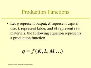
Production Functions Q = F(K, L | given Tech) Or Output = F(Inputs | Chosen Tech)
Production FunctionWhere Only 1 Input Is Variable • Q = F(K, L |T) • But K = K0 (Fixed at level K0 and can’t be changed) • Short-run -> size of the plant; machinery can’t be increased/decreased immediately • -> fixed in the SR • long-run it can be increased or decreased • -> variable in the LR • Look at the short-run for the time being • However L (labor) can be changed very quickly • Layoffs/hiring • So it is variable in both the SR and LR
Production Functions: Total Product, Marginal Product, andAverage Product production function or total product function A numerical or mathematical expression of a relationship between inputs and outputs. It shows units of total product as a function of units of inputs.
FIGURE 7.3Production Function for Sandwiches production function is of the relationship between inputs and outputs. marginal product of labor is the additional output that one additional unit of labor produces.
Buy if We Could Increase K? K0 -> K1 • Able to increase the amount of output each laborer can produce • Increases Total Product at all levels of employment
How about if we could increase both inputs at the same time?
Finally in 2D (really) Isoquants (q1, q2, q3) represent lines of equal (iso) production – or of the same height (product output) from the 3D graph
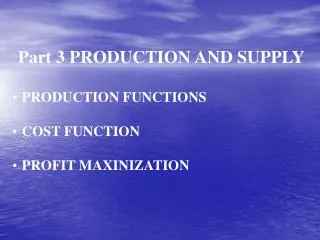
How About Costs? • 2 Input Production Function • Q = F(K, L | T) • Cost • Depend on the quantity of the inputs used • K = # of units of K • L = # of employees (units of L) • Pk, PL = per unit price of Kapital and Labor (wage rate) • Costs of production for a given level of output • C(Q) = PkK + PLL
Choice of Technology Two things determine the cost of production: (1) technologies that are available and (2) input prices. Profit-maximizing firms will choose the technology that minimizes the cost of production given current market input prices.
Factor Prices and Input Combinations: Isocosts FIGURE 7A.3Isocost Lines Showing the Combinations of Capital and Labor Available for $5, $6, and $7 An isocost line shows all the combinations of capital and labor that are available for a given total cost. (PKK) + (PLL) = TC Substituting our data for the lowest isocost line into this general equation, we get isocost line A graph that shows all the combinations of capital and labor available for a given total cost.
Factor Prices and Input Combinations: Isocosts FIGURE 7A.4Isocost Line Showing All Combinations of Capital and Labor Available for $25 One way to draw an isocost line is to determine the endpoints of that line and draw a line connecting them. Slope of isocost line:
Finding the Least-Cost Technology with Isoquants and Isocosts Finding the Least-Cost Combination of Capital and Labor to Produce 50 Units of Output 1. Find the least cost “iso-cost” line that will produce the desired level of output. That is, the least cost (IC) line that touches the 50 output Production isoquant 2. Profit-maximizing firms will minimize costs by producing their chosen level of output where the isoquant is tangent to an isocost line. 3. Here the cost-minimizing technology—3 units of capital and 3 units of labor—is represented by point C. Note: Could produce 50 units at TC = $7; but it would cost more. Could not produce 50 units if your “cost budget” is $5
Finding the minimum cost inputs (quantities) for different levels of output FIGURE 7A.6Minimizing Cost of Production for qX = 50, qX = 100, and qX = 150 FIGURE 7A.7A Cost Curve Shows the Minimum Cost of Producing Each Level of Output Plotting a series of cost-minimizing combinations of inputs—shown in this graph as points A, B, and C— on a separate graph results in a cost curve like the one shown in Figure 7A.7.
The Cost-Minimizing Equilibrium Condition At the point where a line is just tangent to a curve, the two have the same slope. At each point of tangency, the following must be true: Thus, Dividing both sides by PL and multiplying both sides by MPK, we get
isocost line • isoquant • marginal rate of technical substitution • Slope of isoquant: • Slope of isocost line: A P P E N D I X R E V I E W T E R M S A N D C O N C E P T S