Download
1 / 14
140 likes | 238 Vues
Learn how to derive confidence intervals for standard deviation in a random sample, considerations for normality, and using f-distributions for inference.

E N D
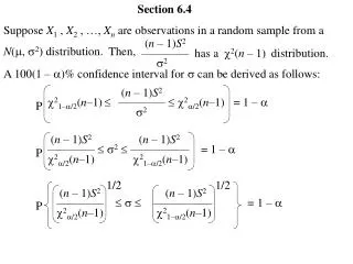
Section 6.4 Suppose X1 , X2 , …, Xn are observations in a random sample from a N(, 2) distribution. Then, (n – 1)S2 ———— has a distribution. 2 2(n – 1) A 100(1 – )% confidence interval for can be derived as follows: (n – 1)S2 21–/2(n–1) ———— 2/2(n–1) = 1 – 2 P (n – 1)S2(n – 1)S2 ———— 2 ————— = 1 – 2/2(n–1) 21–/2(n–1) P 1/2 1/2 (n – 1)S2(n – 1)S2 ———— ————— = 1 – 2/2(n–1) 21–/2(n–1) P
Note: If the random sample does not come from a normal distribution, this confidence interval may not be appropriate, because this confidence interval is sensitive to non-normality. In other words, unlike confidence intervals concerning means, this confidence interval is not robust. If U and V are independent random variables with respective 2(r1) and 2(r2) distributions, then (from Class Exercise 5.2-7, Text Example 5.2-4, or Text Exercise 5.2-2) the random variable has an U / r1 —— V / r2 F = The 100(1 – ) percentile (or the upper 100 percent point) of an f(r1 , r2) distribution is denoted by f(r1 , r2), that is,
1. Find a 95% confidence interval for with the data of Text Exercise 6.2-6. Using the data from Text Exercise 6.2-6, we have Since this is not in the textbook table, we interpolate. Since this is not in the textbook table, we interpolate. 1/2 1/2 (36)11.82(36)11.82 ———— ————— 20.025(36) 20.975(36) 46.98 + [(36–30)/(40–30)](59.34–46.98) 16.79 + [(36–30)/(40–30)](24.43–16.79) 1/2 1/2 (36)11.82(36)11.82 ———— ————— 54.396 21.374 The 95% confidence interval for is 9.600 < < 15.314 We are 95% confident that the standard deviation of the number of colonies in 100 milliliters of water in the west basin is between 9.600 and 15.314.
Note: If the random sample does not come from a normal distribution, this confidence interval may not be appropriate, because this confidence interval is sensitive to non-normality. In other words, unlike confidence intervals concerning means, this confidence interval is not robust. If U and V are independent random variables with respective 2(r1) and 2(r2) distributions, then (from Class Exercise 5.2-7, Text Example 5.2-4, or Text Exercise 5.2-2) the random variable has an U / r1 —— V / r2 F = f distribution with r1 numerator degrees of freedom and r2 denominator degrees of freedom, which we can call an f(r1, r2) distribution. The 100(1 – ) percentile (or the upper 100 percent point) of an f(r1 , r2) distribution is denoted by f(r1 , r2), that is, P[Ff(r1 , r2)] = .
Table VII in Appendix B displays some percentiles for various f distributions. It is useful to observe that 1/F has an f(r2 , r1) distribution. Consequently, P[Ff(r1 , r2)] = P[1/F 1/f(r1 , r2)] = 1 – P[1/F 1/f(r1 , r2)] = P[1/F 1/f(r1 , r2)] = 1 – f1–(r2 , r1) = 1/f(r1 , r2) . Suppose that X1 , X2 , …, Xn are observations in a random sample from a N(X , X2) distribution, that Y1 , Y2 , …, Ym are observations in a random sample from a N(Y , Y2) distribution, and that the two random samples are observed independently of one another. Then, (m–1)SY2 ———— Y2 (m–1) X2SY2 ————————— = —— —— has an distribution. (n–1)SX2Y2SX2 ———— X2 (n–1) f(m – 1 , n – 1) A 100(1 – )% confidence interval for X / Y can be derived as follows:
2. (a) (b) (c) (d) (e) (f) Suppose the random variable F has an f distribution with r1 numerator degrees of freedom and r2 denominator degrees of freedom. If r1 = 5 and r2 = 10, then P(F < 5.64) = 0.99 If r1 = 5 and r2 = 10, then P(F > 4.24) = 0.025 f0.05(4, 8) = 3.84 f0.95(4, 8) = 1/f0.05(8, 4) = 1/6.04 = 0.166 f0.01(8, 4) = 14.80 f0.99(8, 4) = 1/f0.01(4, 8) = 1/7.01 = 0.143
Table VII in Appendix B displays some percentiles for various f distributions. It is useful to observe that 1/F has an f(r2 , r1) distribution. Consequently, P[Ff(r1 , r2)] = P[1/F 1/f(r1 , r2)] = 1 – P[1/F 1/f(r1 , r2)] = P[1/F 1/f(r1 , r2)] = 1 – f1–(r2 , r1) = 1/f(r1 , r2) . Suppose that X1 , X2 , …, Xn are observations in a random sample from a N(X , X2) distribution, that Y1 , Y2 , …, Ym are observations in a random sample from a N(Y , Y2) distribution, and that the two random samples are observed independently of one another. Then, (m–1)SY2 ———— Y2 (m–1) X2SY2 ————————— = —— —— has an distribution. (n–1)SX2Y2SX2 ———— X2 (n–1) f(m – 1 , n – 1) A 100(1 – )% confidence interval for X / Y can be derived as follows:
X2SY2 f1–/2(m – 1 , n – 1) —— —— f/2(m – 1 , n – 1) = 1 – Y2SX2 P 1 X2SY2 ——————— —— —— f/2(m – 1 , n – 1) = 1 – f/2(n – 1 , m – 1) Y2SX2 P 1 SX2X2SX2 ——————— —— —— f/2(m – 1 , n – 1) —— = 1 – f/2(n – 1 , m – 1) SY2Y2SY2 P 1/2 1/2 1 SXXSX ——————— — —— f/2(m – 1 , n – 1) — = 1 – f/2(n – 1 , m – 1) SYYSY P Note: If the random samples do not come from a normal distribution, this confidence interval may not be appropriate, because this confidence interval, like the confidence interval for , is sensitive to non-normality and not robust.
3. Do Text Exercise 6.4-12. 1/2 1/2 1 0.197X0.197 ————— ——— —— f0.05(12 , 15) ——— f0.05(15 , 12) 0.318 Y0.318 1/2 1/2 1 0.197X0.197 —— ——— —— 2.48 ——— 2.62 0.318 Y0.318 The 90% confidence interval for X / Y is 0.383 < X / Y < 0.976 We are 90% confident that the ratio of standard deviations X / Y of mint weights is between 0.383 and 0.976. This confidence interval indicates that there a statistically significant difference in standard deviation, is the afternoon shift. with a larger standard deviation for
4. (a) (b) (c) The random sample X1 , X2 , … , X10 is taken from a N(20, 100) distribution, and the random sample Y1 , Y2 , … , Y16 is taken from a N(8, 100) distribution. The following random variables are defined: T = F1 = F2 = Find each of the following: X– 20 ——— SX / 10 SX2 — SY2 SY2 — SX2 P(– 1.383 < T < 2.262) = 0.975 – 0.10 = 0.875 P(F1 > 3.89) = 0.01 P(F2 > 0.3861) = P(1/ F2 < 2.59) = 0.95
5. (a) (1) Modify the worksheets in the Excel file Confidence_Intervals (created previously) so that the limits of confidence intervals for the variance and standard deviation are displayed, and the limits of confidence intervals for the ratio of two variances and ratio of two standard deviations are displayed. Modify the worksheet named One Sample in the Excel file named Confidence_Intervals as follows: Enter the additional labels displayed in columns B through H, right justify the labels in column E, and underline the labels in cells F15 and H15.
(2) Enter the following formulas respectively in cells F14 and G14: =IF(AND(n>0,$F$13>0,$F$13<1),CHIINV((1-$F$13)/2,n-1),"-") =IF(AND(n>0,$F$13>0,$F$13<1),CHIINV((1+$F$13)/2,n-1),"-") (3) Enter the following formulas respectively in cells F16 and F17: =IF(AND(n>0,$F$13>0,$F$13<1),(n-1)*Variance/$F$14,"-") =IF(AND(n>0,$F$13>0,$F$13<1),(n-1)*Variance/$G$14,"-") (4) Enter the following formula in cell H16: =IF(AND(n>0,$F$13>0,$F$13<1),SQRT(F16),"-") (5) (6) Copy the formula in H16 to H17. Save the file as Confidence_Intervals (in your personal folder on the college network). (b) Use the Excel file Confidence_Intervals to obtain the confidence interval in Text Exercise 6.4-1.
5.-continued (c) (1) Modify the worksheet named Two Sample in the Excel file named Confidence_Intervals as follows: Enter the additional labels displayed in columns B through H, right justify the labels in column E. (2) Enter the following formulas respectively in cells F16 and G16: =IF(AND(n_1>0,n_2>0,$F$15>0,$F$15<1),FINV((1-$F$15)/2,n_2-1,n_1-1),"-") =IF(AND(n_1>0,n_2>0,$F$15>0,$F$15<1),FINV((1+$F$15)/2,n_2-1,n_1-1),"-")
(3) Enter the following formulas respectively in cells F18 and F19: =IF(AND(n_1>0,n_2>0,$F$15>0,$F$15<1),$G$16*Variance_1/Variance_2,"-") =IF(AND(n_1>0,n_2>0,$F$15>0,$F$15<1),$F$16*Variance_1/Variance_2,"-") (4) Enter the following formula in cell H18: =IF(AND(n>0,$F$15>0,$F$15<1),SQRT(F18),"-") (5) (6) Copy the formula in H18 to H19. Save the file as Confidence_Intervals (in your personal folder on the college network). (d) Use the Excel file Confidence_Intervals to obtain the two-sided confidence interval with the 95% confidence level in Text Exercise 6.4-13, instead of the one-sided confidence interval mentioned in part (b). (Open Excel file Data_for_Students in order to copy the data of Exercise 6.4-13.)