Chapter 6: Eigenvalue Problems
Chapter 6: Eigenvalue Problems. Motivation Differential Equations Other Equations. 6.1 Motivation. 6.1 Motivation. Physical Systems are commonly described by ( usually differential) equations involving sets of coupled variables.

Chapter 6: Eigenvalue Problems
E N D
Presentation Transcript
Chapter 6: Eigenvalue Problems Motivation Differential Equations Other Equations
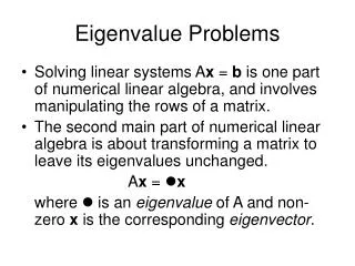
6.1 Motivation 6.1 Motivation Physical Systems are commonly described by ( usually differential) equations involving sets of coupled variables. If the equations are linear and homogeneous (no constant term), they can be looked at as linear transformations, and thus we can express them in matrix form. This, in turn allows us, using diagonalization, to decouple the equations in order to obtain simple solutions. In addition, the solutions to the diagonalized problem exhibit the fundamental characteristics of a physical system. In this chapter, we’ll first work out the solution to the generic problem and then apply the method to 2 concrete examples: an vibrating string and an electrical circuit..
6.2. Differential Equations 6.2-A Linear Differential Equations: General Approach Consider, for instance, the set of n differential equations at right: All dependent variables, x1,…, xn, are all function of the independent variable t; in addition note that the equations are coupled together – variables are interrelated- but they are quite special because only one order of derivative appears – here noted “s”- Thus the approach, although quite general, works only for this type of diff. eq. These equations can be re-written in matrix /vector form as: where: And where the matrix a is: In general this is not so simple. What would make it easy is if the two equations in (1-1) were decoupled, i.e. the first would be an equation involving only x1 and the second equation an equation involving only x2. This can be clearly achieved by diagonalizing the matrix a. Furthermore, in dimensions higher than 2, the solution would be really horrendous, so that diagonalizing the matrix is even more important in that case. And finally, the properties of the system are obscured by the complication of the solution. Diagonalizing the matrix will exhibit the underlying characteristic of a system. By calling P the matrix of the eigenvectors of a, we can define the new variable x such that: Inserting into (1-2) we get: and since P is constant the left hand side can be re-written as:
6.2. Differential Equations And thus finally the equations are decoupled. The solution is very easily found: Example for s=2: then the solution in an exponential: where is the initial value of and is the jth eigenvalue of a. The sign is determined by the physics of the problem (decaying or increasing solution) If we instead have a first order diff eq then s=1 and 6.2-A Linear Differential Equations: General Approach Now, multiplying both sides by on the left we get: Since we know that is the diagonal matrix of the eigenvalues, we have replaced our linear system of equations (1-1) by a decoupled linear system:
6.2. Differential Equations 6.2-A Linear Differential Equations: General Approach This method can also handle derivatives of mixed order Consider for example: Now define: then the above equation becomes: Which together with the definition of x2 becomes a system of two equations: After defining the vector =(the system can now be written in matrix- form as: with the matrix , in our example, given by: So that now the system can be solved as previously. Note that every derivative adds an new variable (in our example the 2nd derivative adds the variable x2
6.2. Differential Equations 6.2-A Linear Differential Equations: General Approach E6.2-1 Consider the equation and 1a. Solve following the same steps as the formal solution above. Find eigenvalues and e.vectors and then P. When finding the matrix P do not get stopped by zero eigenvalue because the eigenvectors of a zero eigenvalue don’t necessarily vanish! 1b. Then get the transformed solution for the Y’s 1c. Then transform back to get the solution in terms of the original y’s and plot in a 2dim graph (y1,y2) the evolution of the solution starting from the point y=(1,-1). E6.2-2 Consider the equation and Solve following the same steps as E6.2-1 E6.2-3 Consider the equation and Write in matrix form and solve. Comment on the solution process! E6.2-4 Consider the equations and . Solve as explained above. To do so follow these steps: 1a. Write equation in matrix form. What is matrix a? 1b. find eigenvalues and eigenvectors of a 1c. Find P 1d. Find P-1 and find x and y in terms of X and Y 1e. Find the solutions for X and Y that stricly decreasing with time (decays) 1f. Then transform back to x and y to find the original variables as a function of time assuming they decay from an original value
6.2. Differential Equations 6.2-B Linear Differential Equations: Example 1 Electrical Circuit Writing that the voltage around each loop of current i1 and i2, is zero we get: In the electrical circuit below the capacitance C1=1microFarad and C2 =2microF are initially charged at VAB =5Volts (say VA>VB). At t=0 the switch S is closed. Find the charge on the capacitors as a function of time. Take R1=R2=100Problem set up: In addition we can write a relationship between q’s and i’s: and So that the equations become: We massage the equations a little to put them in our generic form: Which finally yields:
5.2. Differential Equations 6.2-C Linear Differential Equations: Example 1 cont’d
5.2. Differential Equations 6.2-C Linear Differential Equations: Example 1 cont’d
5.2. Differential Equations 6.2-C Linear Differential Equations: Example 2. Vibrating String & Normal Modes Consider the following 3 masses m attached to a string under tension T. The string is fixed at the ends and massless. The distances are indicated on the drawing. The masses are taken to oscillate in a plane (2dim) and the tension constitutes the net force on the masses (i.e. no gravity is present –outer space - or mg and normal force cancel by letting the masses oscillate in a horizontal plane like a table top) The tension in the rope is assumed to be constant, say T.
5.2. Differential Equations 6.2-C Linear Differential Equations: Example 2. Vibrating String & Normal Modes
5.2. Differential Equations 6.2-C Linear Differential Equations: Example 2. Vibrating String & Normal Modes
5.2. Differential Equations 6.2-C Linear Differential Equations: Example 2. Vibrating String & Normal Modes E6.2-5 Solve the vibrating string problem for 2 masses on a string under tension T. The masses are located at a distance d from the fixed ends of the string, and are separated by a distance 2d. Find the general solution from the position of the masses as a function of time and find the normal modes of the system.

