Download
1 / 22
220 likes | 407 Vues
Inflation-Unemployment Tradeoff. Lecture 12. The Equation for Wage Inflation. RW=A0+RP1+RQ-A1*(U-U@VOL) The rate of change of wages (RW) equals the rate of change in prices (RP) in the past year (“1”) as a proxy for expected inflation plus productivity growth

E N D
Inflation-Unemployment Tradeoff Lecture 12
The Equation for Wage Inflation RW=A0+RP\1+RQ-A1*(U-U@VOL) The rate of change of wages (RW) equals • the rate of change in prices (RP) in the past year (“\1”) as a proxy for expected inflation • plus productivity growth • minus an adjustment for the existence of involuntarily unemployed workers:total unemployment (U) - voluntary (U@VOL) • plus a constant (A0) other factors not specifically defined here • Note: many coefficients expected to equal 1
The Equation for Wage Inflation Dependent Variable: %ch of Wage per Hour Method: Least Squares Date: 03/24/00 Time: 14:16 Sample(adjusted): 1976 1999 Variable Coefficient Std. Error t-Statistic C 0.002 0.004 0.62 (U-UFE)/100 -0.45 0.10 4.34 Average inflation of recent years: %ch(CPI)+%ch(CPI(-1))+%ch(CPI(-2)))/3 0.81 0.05 16.36 Average productivity growth: %ch(QPERH(-1))+%ch(QPERH(-2)))/2 where QPERH=Output per Hour 0.47 0.15 3.02 R-squared 0.936629 S.E. of regression 0.0055 Note: The coefficient for average price inflation over the past 3 years is just under 1. The coefficient for recent productivity growth is only about .5
A Companion Equation for Price Inflation • If prices are a simple “mark-up” on wages adjusted for productivity (QperH) (wages divided by productivity = unit labor costs).. • P = K * W/QperH • hence RP = RK + R(W/QperH) • ..and this markup could fall when the economy is sluggish • RK = B0 - B1 * (U-U@VOL) • Then: RP = B0 - B1 * (U-U@VOL) + R(W/QperH) • Additional Factors Need to be Added for Aggregate Supply Shocks Such as Oil or Other Imported Goods Prices
A Companion Equation for Price Inflation Dependent Variable: @PCH(CPI) consumer price inflation Method: Least Squares Date: 03/24/00 Time: 14:37 Sample(adjusted): 1977 1999 Included observations: 23 after adjusting endpoints Variable Coefficient Std. Error t-Statistic C 0.02 0.003 7.86 NEWCPI Definition Shift -0.006 0.004 -1.64 @PCH(ECIWSP/JQPERMH) current wages relative to productivity=unit labor costs .58 0.08 7.42 @PCH(ECIWSP(-1)/JQPERMH(-1)) lagged wages relative to productivity 0.26 0.07 3.79 @PCH(IMPORTPRICES/(ECIWSP/JQPERMH)) import prices rel. to. unit labor costs 0.12 0.03 3.47 @PCH(WPI05/(ECIWSP/JQPERMH)) energy prices rel. to unit labor costs 0.07 0.02 3.21 R-squared 0.969657 S.E. of regression 0.006245 Consumer price inflation was not found to be related to the unemployment rate, so this factor is not included The sum of the coefficients on unit labor costs is also just under the expected value of 1.0. The
The Final Form Model of Price Inflation If we assume the three key coefficients actually equal 1( if we had perfect measures of the concepts): • price inflation affecting wages • wage inflation affecting prices) • And productivity affecting both wages (positively) and price(negatively), then: (1) RP = RW-RQ+Supply Shocks AND, EARLIER, (2) RW=RP\1+ RQ+ A0-A1*(U-U@VOL) Substituting (2) into (1) yields: RP=RP\1+ RQ+ A0-A1*(U-U@VOL) -RQ+Supply Shocks =RP\1+ A0-A1*(U-U@VOL) +Supply Shocks (Note: Productivity is neutral in this formulation) OR, RP-RP\1 =THE CHANGE IN INFLATION (i.e the acceleration in prices) = A0-A1*(U-U@VOL) +Supply Shocks
The Final Form Model of Wage and Price Inflation OR, RP-RP\1 =THE CHANGE IN INFLATION (i.e the acceleration in prices) = A0-A1*(U-U@VOL) +Supply Shocks THE CHANGE IN INFLATION = A FUNCTION OF THE ADJUSTED LEVEL OF UNEMPLOYMENT, plus or minus any external supply shocks A stable, low rate of inflation is a valuable attribute of an economy: it promotes good decision making because economic life is predictable and unbiased by continually changing prices If inflation is constant, RP = RP\1 and the price level is “non-accelerating”, we can compute the associated “non-accelerating rate of unemployment” or “NAIRU”. For this to hold, 0= (A0) - (A1) * (U-U@VOL) Hence, U(NAIRU) = U@VOL + A0 / A1 Note that in the estimated equations, the constant terms were very close to zero, thus U(NAIRU) is the U@VOL.
The Link Between Unemployment and Real Output RP-RP\1 = (A0) -(A1)*(U-U@VOL) + Supply Shocks is a solid relationship. We need to create a parallel relationship between the change in inflation and output to tie into the IS-LM model. Thus, we need to understand the relationship between output and unemployment. By approximate definition, the Change in the Unemployment rate = %ch (labor force)- %ch(employment) and %ch(employment) = %ch(GDP) minus %ch(productivity) Hence Change in U = %ch (labor force) - %ch(GDP) + %ch(productivity) When demand (real GDP) rises, employers must increase output by either raising the number of employees (E) or the productivity of those already employed. In the short-run context of IS-LM analysis, the applied technology cannot change and the capital stock is also fixed. However, assembly lines can be run somewhat faster, more overtime hours can be used, employees can be asked to be more efficient, etc. Thus each 1% short-run increase in demand for GDP tends to require only a fractional % increase in employment. Also, when the economy cycles, participation in the labor force changes in response---more people look for work when times are thought to be good. Therefore the % change in the unemployment rate is less than the % change in output, but a close relationship is likely.
Note: 3% GDP Growth => No U Rate Change, and Each Extra 1% Growth =>1/2% U Rate Drop
The Link Between Unemployment and Real Output • The cyclical relationship between unemployment and real growth is known as Okun’s Law: • the change in Unemployment Rate= about half the growth rate differencebetween potential and actual GDP growth • or, the level of the Unemployment Rate= about half the % gap between potential and actual GDP
Note: 1% GDP Growth => Fractionally Higher: • Labor Force Growth, • Employment Growth, and • Productivity Growth
The Link Between Full Employment NAIRU and Real Output • The unemployment rate reflects the difference between the demand for and the supply of labor. • The demand for labor is the number of employees (E) needed, with a given productivity (GDP/E) to produce a given output (GDP) • or, E = GDP / (GDP/E) • The supply of labor is the number of workers (L) seeking to work at a given real wage • The Potential output they can produce in a “Fully Employed economy” = “an economy operating at the “NAIRU” is called “Potential GDP” (GDP@ FE) • GDP@FE=L* (1-NAIRU) * (Productivity)
The Link Between Unemployment and Real Output • The cyclical relationship between unemployment and real growth is known as Okun’s Law: • the change in Unemployment Rate= about half the growth rate differencebetween potential and actual GDP growth • or, the level of the Unemployment Rate= about half the % gap between potential and actual GDP
The Full Links Among:Inflation, Unemployment and Real Output The critical relationships are: 1. Thechange in inflation responds (with a negative derivative) to the unemployment rate 2. The unemployment rate responds (with a negative derivative) to the GDP level (for any given capital stock etc determining GDP@FE) Therefore, 3. The change in inflation responds (with a positive derivative) to the GDP level, given GDP@FE change in inflation GDP level GDP@FE
The Full Links Among:Inflation, Unemployment and Real Output The change in inflation responds (with a positive derivative) to the GDP level, given GDP@FE. A favorable external shock, such as a drop in oil prices or imported goods prices, effective reduces the NAIRU (the unemployment rate required to keep inflation unchanged), and thereby raises GDP@FE. Note: An increase in the rate of growth of productivity does not change NAIRU, if as shown the positive reaction of wages to productivity is the same absolute magnitude (but opposite sign) as the reaction of price to prodcutivity. However, a rise the rate of growth of productivity does boost potential full employment output: quite naturally if the same proportion of the labor force is employed (unchanged NAIRU) but each employee produces more, then full-employment output is higher. GDP@FE with NAIRU (1) change in inflation GDP level 0 GDP@FE with NAIRU (2)
The Determination of Trend Potential GDP GDP@FE expands in predictable ways (see Basic Growth lectures) • GDP requires capital, labor, and technology • If we use a narrow definition of capital as physical capital, then trend GDP growth is the weighted average of capital and labor growth rates, plus the total factor productivity growth created by advancing technology • A broader definition of capital changes the defined labor and capital growth rates and hence the residual left for technology
Recall the Determinants of Labor Productivity • What enables an employee to produce more or less per hour? • The “state of the art” potentially available (the production possibility frontier”). • His/ Her own education and training to absorb the state of the art. • The quantity and quality of available, complementary “tools” such as computers, assembly machines.
The Determinants of Labor Productivity • What “infrastructure” can the nation provide to influence: • the level of output in a workplace? • education, health, attitudes toward work, regulation, taxation • the efficiency of “connections” between workplaces? • communication, transportation, common language, anti-monopoly regulation, global access
The Determinants of Labor Productivity • Economists canrefer to almost all of these factors as simply different types of “capital” • “Capital” in this context simply means something that is long-lasting and not used up by the process of production • More narrowly, “capital” sometimes only means tangible goods such as equipment, buildings, highways
The Determinants of Labor Productivity • Types of Capital • Tangible equipment and structures • Human, from brains through brawn • Technological, e.g. accumulated R&D • Infrastructure, i.e. tangible goods not owned by one enterprise