Download
1 / 20
200 likes | 279 Vues
IE733 – Prof. Jacobus 4 a Aula Potenciais de Contato e Introdução ao MOSFET. Potencial de Contato. Metal-metal: Metal - M (eV) Ag 5.1 Al 4.1 Au 5.0 Cu 4.7 Mg 3.4 Ni 5.6 Pd 5.1 Pt 5.7. Metal-Si. onde:. Da condição de contorno, (0)=0, obtemos:. Com aplicação de tensão:.

E N D
IE733 – Prof. Jacobus4a AulaPotenciais de Contato eIntrodução ao MOSFET.
Potencial de Contato • Metal-metal: • Metal - M(eV) • Ag 5.1 • Al 4.1 • Au 5.0 • Cu 4.7 • Mg 3.4 • Ni 5.6 • Pd 5.1 • Pt 5.7
Da condição de contorno, (0)=0, obtemos:
Formação de contato ôhmico: a) M < S
Nomenclatura de Tsividis: Potencial de contato: J1,J2= J1-J2, (onde =potencial) Caso J1 < J2, (onde =energia=função trabalho):
Conhecendo os valores de J em relação ao Si intrínseco, Podemos calcular J1,J2 entre dois materiais quaisquer:
Potencial de contato de Al p/ Si-p (NA=1015 cm-3) Potencial de contato de Si-p (NA= 1014 cm-3) p/ Si-n (ND=1016 cm-3) Exemplos:
Vários materiais em série: Medida com voltímetro: Inserindo uma fonte de tensão:
Introdução ao Transistor MOS Lilienfeld, 1928 – um homem muito à frente do seu tempo!
CMOS = nMOS + pMOS Algumas características: W = WM-W L = LM-L IG 0 IJR 1 pA/área mínima em RT (aumenta ~ 2x a cada 8 a 10 C) VDS < BV
Para VGS < VT superfície do pistão > nível da fonte: ns(elétrons) moléculas vapor IDS fluxo H2O (por difusão) nH2O(h) e-h Portanto: fluxo e-h
Características de MOSFET Tensão de limiar clássica: