Regression
Regression. Review and Extension. The Formula for a Straight Line. Only one possible straight line can be drawn once the slope and Y intercept are specified The formula for a straight line is: Y = b x + a Y = the calculated value for the variable on the vertical axis a = the intercept

Regression
E N D
Presentation Transcript
Regression Review and Extension
The Formula for a Straight Line • Only one possible straight line can be drawn once the slope and Y intercept are specified • The formula for a straight line is: • Y = bx + a • Y = the calculated value for the variable on the vertical axis • a = the intercept • b = the slope of the line • X = a value for the variable on the horizontal axis • Once this line is specified, we can calculate the corresponding value of Y for any value of X entered
The Line of Best Fit • Real data do not conform perfectly to a straight line • The best fit straight line is that which minimizes the amount of variation in data points from the line • Note that this is a key idea, you get to choose how you want to minimize some estimate of variability about a regression line • The typical approach is the least squares method • The equation for this line can be used to predict or estimate an individual’s score on Y on the basis of his or her score on X
Least Squares Modeling • When the relation between variables are expressed in this manner, we call the relevant equation(s) mathematical models • The intercept and weight values are called the parameters of the model. • We’ll assume that our models are causal models, such that the variable on the left-hand side of the equation is being caused by the variable(s) on the right side.
Terminology • The values of Y in these models are often called predicted values, sometimes abbreviated as Y-hat or • They are the values of Y that are implied or predicted by the specific parameters of the model.
Parameter Estimation • In estimating the parameters of our model, we are trying to find a set of parameters that minimizes the error variance. In other words, we want the sum of the squared residuals to be as small as it possibly can be. • The process of finding this minimum value is called least-squares estimation.
Least-squares estimation • The relevant equations:
Estimates of a and b • Estimating the Slope (the regression coefficient) • Estimating the Y intercept • These calculations ensure that the regression line passes through the point on the scatterplot defined by the means of X and Y
Standardized regression coefficient • Standardized slope is often given in output, and will have added usefulness within multiple regression • When normally distributed scores are changed into Z scores the mean is 0 and standard deviation is 1. Referring to our previous formula: • So r would be equal to the slope, and interpreted as 1 sd unit of change in X leads to a b sd unit change in Y
What can the model explain? • Total variability in the dependent variable (observed – mean) comes from two sources • Variability predicted by the model i.e. what variability in the dependent variable is due to the independent variable • How far off our predicted values are from the mean of Y • Error or residual variability i.e. variability not explained by the independent variable • The difference between the predicted values and the observed values S2y S2 S2(yi - i) Total variance = predicted variance + error variance
R-squared - the coefficient of determination • The square of the correlation, r², is the fraction of the variation in the values of y that is explained by the regression of y on x • Conceptually: • R²= variance of predicted values y variance of observed values y
R2 • The shaded portion shared by the two circles represents the proportion of shared variance: the larger the area of overlap, the greater the strength of the association between the two variables A Venn Diagram Showing r2 as the Proportion of Variability Shared by Two Variables (X and Y)
Interpreting regression summary • Intercept • Value of Y if X is 0 • Often not meaningful, particularly if it’s practically impossible to have an X of 0 (e.g. weight) • Slope • Amount of change in Y seen with 1 unit change in X • Standardized regression coefficient • Amount of change in Y seen in standard deviation units with 1 standard deviation unit change in X • In simple regression it is equivalent to the r for the two variables • Standard error of estimate • Essentially the standard deviation of the residuals • The difference involves dividing by df residuals for the model (see) vs. n-1 (sd) • As R2 goes up, it goes down • Statistical significance of the model • R2 • Proportion of variance explained by the model
The Caution of Causality • Correlation does not prove causality, but… • One can’t establish causality without correlation • One thing to remember is that just because things look good for your model, other models may be as viable or even better
Assumptions in regression • For starters: • Linear relationship between the independent and dependent variable • Residuals are normally distributed • Residuals are independent
Heteroscedasticity • We also assume residuals have the same variance about the regression line • Homoscedasticity • Example of heteroscedasticity
Interval measures and measurement without error • Ordinal variables are not to be used as the differences among levels is not constant • But we like our Likerts! • Most suggest that at least 5 to lessen the impact of ordinal differences (7 or more better) • Measurement without error • Must have reliable measures involved • More random error will lead to larger error variance • Less reliable, smaller R2
Violating assumptions • Usual situation • Slight problems may not result in much change in type I error • However, type II will be a major concern with even modest violations • With multiple violations, type I may also suffer • Additional assumptions will be made for multiple independent variables
Outliers • As outliers can greatly influence r, they will naturally influence any analysis using it • Detecting and dealing with outliers is a part of the process of regression analysis • One issue is distinguishing univariate vs. multivariate outliers • While a data point might be an outlier on a variable, it may not be as far as the model goes • Conversely, what might be an outlier for the model, might not have it’s individual variable values noted as outliers
Robust Regression • A single unusual point can greatly distort the picture regarding the relationship among variables • Heteroscedasticity, even in ‘normal’ situations, inflates the standard error of estimate and decreases our estimate of R2 • Nonnormality can hamper our ability to come up with useful interval measures for slopes
Robust Regression • While least squares regression performs well in general if we are conducting hypothesis testing regarding independence, it is poor at detecting associations in less than ideal circumstances • What we would like are methods that perform well in a variety of circumstances, and compete well with least-squares regression under ideal conditions • To be discussed: • Theil-Sen Estimator • Regression via robust correlation • L regression • Least trimmed squares • Least trimmed absolute value • Least median of squares • M-estimators • Deepest regression line
Theil-Sen Estimator • For any pair of data points regarding a relationship between two variables, we can plot those 2 points, produce a line connecting them, and note its slope • E.g. if we had 4 data points we could calculate 6 slopes • X = 1,2,3,4 • Y = 5,7,11,15 • If each of those slopes is weighted by the squared difference in X values for the appropriate points, the weighted average of all our slopes created would be the LS slope for the model • E.g. Create a line for the points, (1,5) and (2,7) • Slope = 2 • Weight by (1-2)2 • What if instead of a weighted average, the median of those slopes is chosen as our model slope estimate? • That in essence is the Theil-Sen estimator
Theil-Sen Estimator • Advantages • Competes with LS regression in ideal conditions • More resistant • Reduced standard error in problematic situations, e.g. heteroscedasticity • We can, using the percentile bootstrap method, calculate CIs as well *It has been shown that the median approach here performs better than trimming less
Regression via robust correlation • We could simple replace our regular r with a more robust estimate • This is possible but more work needs to be done to figure out which approaches might be more viable, and it appears bias might be a problem in some cases with this approach (e.g. heteroscedastic situations using a winsorized r)
Least Absolute Value • Instead of minimizing the sum of the squared residuals, we could choose a method that attempts to minimize the sum of the absolute residuals • L1 regression • Problem: while protecting against outliers on Y, it does not for values of on the predictor
Least Trimmed Squares • The least trimmed squares approach involves trimming the smallest and largest residuals • So if h is the amount of values left after trimming and • Then the goal would be to minimize the sum of the squared residuals of the remaining data • Note again that optimal trimming amount is about ~.2
S-plus menu example • The first two show the standard menu availability of least trimmed squares regression • The last uses the robust library
Least Trimmed Absolute Value • Same approach, but rather than minimize the trimmed squared residuals, we minimize the sum of the absolute residuals remaining after trimming • This may be preferable to LTS in heteroscedastic situations
Least Median of Squares • Find the slope and intercept that minimizes the median of the squared residuals • Doesn’t seem to perform as well generally as other robust approaches
M-estimators • In general, regression using M-estimators minimize the sum of some function of the residuals • Where ξ is a function used to guard against outliers and heteroscedasticity • E.g. ξ(r1) = r2 would give us our regular LS result • Although there are many M-estimator approaches one might be able to choose from given the newness of the approach in general and our relative lack of research regarding it, Wilcox suggest the adjusted M-estimator seems to work well in practical situations • First checks for “bad” leverage points and may ignore in estimate of slope and intercept
Leverage points • Leverage is one aspect of ‘outlierness’ that we’ll mention here but come back to later • It is primarily concerned with outliers among predictors • E.g. Mahalanobis distance • Good leverage points may be extreme with regard to predictors but is not an outlier with regard to the model • In LS, it can decrease the standard error • Bad leverage points are extreme and would not lie close to a line that would fit most of the data well, and have a profound effect on your estimate of the slope
Deepest regression line • One of the more recent developments, and may be of practical use as it is researched further • It is really more about linear fit (i.e. matching parameters to data) as opposed to focus on the observations/residuals themselves • Depth is the number of observations that would need to be removed to make the data ‘nonfit’ • Appears to have a breakdown point of about 1/3 regardless of the number of predictors
Summary • In single predictor situations, alternatives are available that perform well in ideal situations, and much better than the LS approach in others • Theil-Sen in particular • While we have kept to the single predictor, this will typically never be our research situation in using regression analysis • These methods can also be generalized to the multiple predictor setting, but their breakdown point (i.e. resistance advantage) decreases as more predictors enter into the equation
Summary • Again we call on the Tukey suggestion • “… just which robust/resistant methods you use is not important – what is important is that you use some. It is perfectly proper to use both classical and robust/resistant methods routinely, and only worry when they differ enough to matter. But when they differ, you should think hard.” • A general approach: • Check for linearity • Perhaps using a smoother • If ok there, then use an estimator with a breakdown point of about .2-.3, and compare with LS output • If notable differences between LS and robust exist, figure out why and determine which is more appropriate • If assumptions are tenable and little difference between LS and robust exists, feel comfortable going with the LS output

