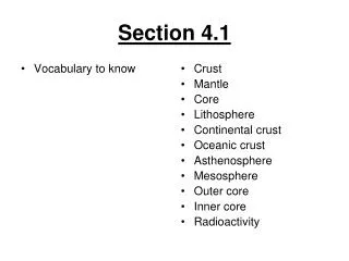
Section 4.1
Section 4.1. Probability Distributions. Section 4.1 Objectives. Distinguish between discrete random variables and continuous random variables Construct a discrete probability distribution and its graph Determine if a distribution is a probability distribution

Section 4.1
E N D
Presentation Transcript
Section 4.1 Probability Distributions
Section 4.1 Objectives • Distinguish between discrete random variables and continuous random variables • Construct a discrete probability distribution and its graph • Determine if a distribution is a probability distribution • Find the mean, variance, and standard deviation of a discrete probability distribution • Find the expected value of a discrete probability distribution
Random Variables Random Variable • Represents a numerical value associated with each outcome of a probability distribution. • Denoted by x • Examples • x = Number of sales calls a salesperson makes in one day. • x = Hours spent on sales calls in one day.
Random Variables Discrete Random Variable • Has a finite or countable number of possible outcomes that can be listed. • Example • x = Number of sales calls a salesperson makes in one day. x 0 1 2 3 4 5
Random Variables Continuous Random Variable • Has an uncountable number of possible outcomes, represented by an interval on the number line. • Example • x = Hours spent on sales calls in one day. x 0 1 2 3 … 24
Example: Random Variables Decide whether the random variable x is discrete or continuous. xx = The number of Fortune 500 companies that lost money in the previous year. Solution:Discrete random variable (The number of companies that lost money in the previous year can be counted.) {0, 1, 2, 3, …, 500}
Example: Random Variables Decide whether the random variable x is discrete or continuous. xx = The volume of gasoline in a 21-gallon tank. Solution:Continuous random variable (The amount of gasoline in the tank can be any volume between 0 gallons and 21 gallons.)
Discrete Probability Distributions Discrete probability distribution • Lists each possible value the random variable can assume, together with its probability. • Must satisfy the following conditions: In Words In Symbols 0 ≤ P (x) ≤ 1 • The probability of each value of the discrete random variable is between 0 and 1, inclusive. • The sum of all the probabilities is 1. ΣP(x) = 1
Constructing a Discrete Probability Distribution Let x be a discrete random variable with possible outcomes x1, x2, … , xn. • Make a frequency distribution for the possible outcomes. • Find the sum of the frequencies. • Find the probability of each possible outcome by dividing its frequency by the sum of the frequencies. • Check that each probability is between 0 and 1, inclusive, and that the sum of all probabilities is 1.
Example: Constructing a Discrete Probability Distribution An industrial psychologist administered a personality inventory test for passive-aggressive traits to 150 employees. Individuals were given a score from 1 to 5, where 1 was extremely passive and 5 extremely aggressive. A score of 3 indicated neither trait. Construct a probability distribution for the random variable x. Then graph the distribution using a histogram.
Solution: Constructing a Discrete Probability Distribution • Divide the frequency of each score by the total number of individuals in the study to find the probability for each value of the random variable. • Discrete probability distribution:
Solution: Constructing a Discrete Probability Distribution This is a valid discrete probability distribution since Each probability is between 0 and 1, inclusive,0 ≤ P(x)≤ 1. The sum of the probabilities equals 1, ΣP(x) = 0.16 + 0.22 + 0.28 + 0.20 + 0.14 = 1.
Solution: Constructing a Discrete Probability Distribution • Histogram Because the width of each bar is one, the area of each bar is equal to the probability of a particular outcome.
Mean Mean of a discrete probability distribution • μ = ΣxP(x) • Each value of x is multiplied by its corresponding probability and the products are added.
Example: Finding the Mean The probability distribution for the personality inventory test for passive-aggressive traits is given. Find the mean score. Solution: μ = ΣxP(x)= 2.94
Variance and Standard Deviation Variance of a discrete probability distribution • σ2 = Σ(x – μ)2P(x) Standard deviation of a discrete probability distribution
Example: Finding the Variance and Standard Deviation The probability distribution for the personality inventory test for passive-aggressive traits is given. Find the variance and standard deviation. ( μ = 2.94)
Solution: Finding the Variance and Standard Deviation Recall μ = 2.94 Variance: σ2 = Σ(x – μ)2P(x) = 1.616 Standard Deviation:
Expected Value Expected value of a discrete random variable • Equal to the mean of the random variable. • E(x) = μ = ΣxP(x)
Example: Finding an Expected Value At a raffle, 1500 tickets are sold at $2 each for four prizes of $500, $250, $150, and $75. You buy one ticket. What is the expected value of your gain?
Solution: Finding an Expected Value • To find the gain for each prize, subtractthe price of the ticket from the prize: • Your gain for the $500 prize is $500 – $2 = $498 • Your gain for the $250 prize is $250 – $2 = $248 • Your gain for the $150 prize is $150 – $2 = $148 • Your gain for the $75 prize is $75 – $2 = $73 • If you do not win a prize, your gain is $0 – $2 = –$2
Solution: Finding an Expected Value • Probability distribution for the possible gains (outcomes) 22 of 63
Section 4.1 Summary • Distinguished between discrete random variables and continuous random variables • Constructed a discrete probability distribution and its graph • Determined if a distribution is a probability distribution • Found the mean, variance, and standard deviation of a discrete probability distribution • Found the expected value of a discrete probability distribution