Implicit Scheme for Image Segmentation using Level Set Framework
Learn about improving image segmentation using a topological change with an implicit scheme. Explore the transition from active contours to level set framework for evolving the level set function efficiently.

Implicit Scheme for Image Segmentation using Level Set Framework
E N D
Presentation Transcript
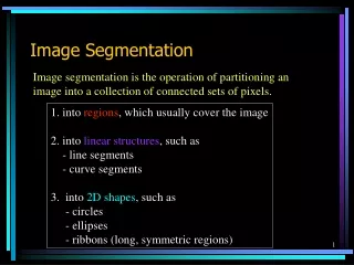
Image Segmentation February 27, 2007
Implicit Scheme is considerably better with topological change. • Transition from Active Contours: • contour v(t) front (t) • contour energy forces FA FC • image energy speed function kI • Level set: • The level set c0 at time t of a function (x,y,t) is the set of arguments { (x,y) , (x,y,t) = c0 } • Idea: define a function (x,y,t) so that at any time, (t) = { (x,y) , (x,y,t) = 0 } • there are many such • has many other level sets, more or less parallel to • only has a meaning for segmentation, not any other level set of
Level Set Framework (x,y,t) 0 0 0 5 7 6 5 4 4 4 3 2 0 1 1 1 2 0 3 4 5 6 5 4 3 3 3 2 0 1 1 2 0 3 4 5 4 3 0 2 2 0 0 2 1 -1 -1 -1 0 1 2 3 4 3 0 2 1 1 1 -1 -2 -2 -2 -1 0 1 2 3 2 1 0 -1 -2 -3 -3 0 -2 -1 1 2 0 2 1 0 -1 -1 -1 -2 -3 -3 0 -2 -1 1 2 3 2 1 -1 0 -2 -2 -3 -3 -2 -1 0 1 2 3 4 2 1 -1 0 -2 -2 0 0 -2 0 -2 -1 0 1 2 3 4 5 3 2 1 -1 -1 -1 -1 0 -1 0 1 2 3 4 5 -2 4 3 2 1 -1 -1 1 2 3 4 5 4 3 2 1 1 1 1 1 2 3 4 5 6 5 4 3 2 2 2 2 1 1 2 3 4 5 6 (x,y,t) (t) Usual choice for : signed distance to the front (0) - d(x,y, ) if (x,y) inside the front (x,y,0) = 0 “ on “ d(x,y, ) “ outside “
Level Set 7 0 0 0 6 5 4 4 4 3 0 2 1 1 1 0 2 3 4 5 6 5 4 3 3 3 0 2 1 1 2 0 3 4 5 4 3 2 0 2 0 0 2 1 -1 -1 -1 1 0 2 3 4 3 2 0 1 1 1 -1 -2 -2 -2 -1 0 1 2 3 2 1 0 -1 -2 -3 -3 -2 0 -1 1 2 2 1 0 -1 -1 -1 -2 -3 -3 0 -2 -1 1 2 3 7 6 5 4 4 4 3 2 2 1 3 1 4 1 5 2 1 -1 0 -2 -2 -3 -3 -2 -1 0 1 2 3 4 6 5 4 3 3 3 2 0 -1 2 0 3 0 4 1 2 1 -1 0 -2 -2 0 -2 0 0 -2 -1 1 0 2 3 4 5 5 4 3 2 2 2 -2 1 -1 -1 2 -1 3 0 1 3 2 1 -1 -1 -1 -1 0 -1 0 1 2 3 4 5 4 3 2 1 1 -2 1 -2 0 -2 -1 2 -1 0 1 4 3 2 1 -1 -1 1 2 3 4 3 2 1 0 -2 0 -3 0 -3 -1 -2 2 -1 0 1 5 4 3 2 1 1 1 1 1 2 3 4 5 2 1 0 -2 -1 -3 -1 -3 -1 -2 2 -1 3 0 1 6 5 4 3 2 2 2 2 1 1 2 3 4 5 6 2 -2 1 -2 0 -3 -1 -3 -2 2 -1 3 0 4 1 2 -2 1 -2 1 -2 0 -2 2 0 3 0 4 1 5 (x,y,t+1) = (x,y,t) + ∆(x,y,t) 3 2 -3 1 0 -1 1 -1 0 2 3 1 4 1 5 4 3 2 -2 0 -1 0 1 2 1 2 0 3 0 4 5 4 3 2 0 0 1 1 0 2 -1 4 0 5 1 6 5 4 3 2 2 2 1 2 0 4 0 5 1 6 • no movement, only change of values • the front may change its topology • the front location may be between samples (x,y,t)
Level Set • Segmentation with LS: • Initialise the front (0) • Compute (x,y,0) • Iterate: • (x,y,t+1) = (x,y,t) + ∆(x,y,t) • until convergence • Mark the front (tend)
Equation for Front Propagation product of influences spatial derivative of (x,y,t+1) - (x,y,t) smoothing “force” depending on the local curvature (contour influence) extension of the speed function kI(image influence) constant “force” (balloon pressure) link between spatial and temporal derivatives, but not the same type of motion as contours!
Equation for Front Propagation ^ kI ^ kI (x,y) = kI(x’,y’) where (x’,y’) is the point in the front closest to (x,y) ^ ( such a kI (x,y) depends on the front location ) • Speed function: • kI is meant to stop the front on the object’s boundaries • similar to image energy: kI(x,y) = 1 / ( 1 + || I (x,y) || ) • only makes sense for the front (level set 0) • yet, same equation for all level sets • extend kI to all level sets, defining • possible extension:
Algorithm 7 7 0 0 0 0 0 0 0 0 0 6 6 5 5 4 4 4 4 4 4 3 3 0 0 2 0 2 1 1 1 1 1 1 0 2 0 2 0 3 3 4 4 5 5 6 6 5 5 4 4 3 3 3 3 3 3 0 0 2 0 2 1 1 1 1 2 0 2 0 0 3 3 4 4 5 5 4 4 3 3 0 0 2 0 2 2 0 2 0 0 0 0 0 2 2 1 1 -1 -1 -1 -1 -1 -1 0 0 1 1 0 2 2 3 3 4 4 3 3 0 2 2 0 0 1 1 1 1 1 1 -1 -1 -2 -2 -2 -2 -2 -2 -1 -1 0 0 0 1 1 2 2 3 3 2 2 0 1 0 0 1 -1 -1 -2 -2 -3 -3 -3 -3 -2 0 -2 0 0 -1 -1 1 1 2 2 2 2 1 1 0 0 0 -1 -1 -1 -1 -1 -1 -2 -2 -3 -3 -3 -3 0 0 -2 -2 0 -1 -1 1 1 2 2 3 3 7 6 5 4 4 4 3 2 0 2 1 3 1 4 1 5 2 2 1 1 0 -1 0 -1 0 -2 -2 -2 -2 -3 -3 -3 -3 -2 -2 0 0 -1 -1 0 1 1 2 2 3 3 4 4 6 5 4 3 3 3 2 0 0 0 -1 2 3 4 1 2 2 1 1 -1 -1 -2 0 0 -2 0 0 -2 -2 0 0 0 -2 -2 0 0 0 -2 0 -2 0 -1 -1 1 1 0 0 0 2 2 3 3 4 4 5 5 5 4 3 2 2 2 0 -2 1 -1 0 -1 2 -1 3 1 3 3 2 2 1 1 -1 -1 -1 -1 -1 -1 -1 -1 -1 0 0 0 -1 0 0 0 1 1 2 2 3 3 4 4 5 5 4 3 2 0 1 1 -2 1 -2 -2 -1 0 2 -1 1 4 4 3 3 2 2 1 1 -1 -1 -1 -1 1 1 2 2 3 3 4 4 3 2 0 0 0 1 -2 -3 -3 -1 -2 0 2 -1 1 5 5 4 4 3 3 2 2 1 1 1 1 1 1 1 1 1 1 2 2 3 3 4 4 5 5 2 0 1 -2 -1 -3 -1 -3 -1 -2 0 2 -1 3 1 6 6 5 5 4 4 3 3 2 2 2 2 2 2 2 2 1 1 1 1 2 2 3 3 4 4 5 5 6 6 2 0 -2 1 -2 -3 -1 -3 -2 0 2 -1 3 4 1 2 0 -2 1 -2 1 -2 -2 0 0 2 3 4 1 5 3 2 0 -3 1 0 -1 1 -1 2 3 1 4 1 5 4 3 2 0 -2 0 -1 0 0 1 2 1 2 3 4 5 4 3 2 0 0 0 1 0 1 2 -1 4 5 1 6 5 4 3 2 2 2 0 1 0 2 4 5 1 6 1. compute the speed kI on the front extend it to all other level sets 2. compute (x,y,t+1) = (x,y,t) + ∆(x,y,t) 3. find the front location (for next iteration) modify (x,y,t+1) by linear interpolation (x,y,t)
Narrow band extension 0 0 0 0 2 1 1 1 2 0 0 2 1 1 2 0 2 0 2 0 0 2 1 -1 -1 -1 1 0 2 2 0 1 1 1 -1 -2 -2 -2 0 -1 1 2 2 0 1 -1 -2 0 -2 -1 1 2 2 1 0 -1 -1 -1 -2 -2 0 -1 1 2 2 1 0 -1 -2 -2 -2 0 -1 1 2 2 1 -1 0 -2 0 -2 0 -2 0 -2 -1 0 1 2 2 1 -1 -1 -1 -1 -1 0 0 1 2 2 1 -1 -1 1 2 2 1 1 1 1 1 2 2 2 2 2 1 1 2 • Weaknesses of algorithm 1 • update of all (x,y,t): inefficient, only care about the front • speed extension: computationally expensive • Improvement: • narrow band: only update a few level sets around • other extended speed: kI(x,y) = 1 / ( 1 + || I(x,y)|| ) ^
Narrow band extension 0 0 0 2 0 1 1 1 0 2 0 2 1 1 0 2 0 2 0 2 2 0 1 -1 -1 -1 1 0 2 2 0 1 1 1 -1 -2 -2 -2 -1 0 1 2 2 1 0 -1 -2 0 -2 -1 1 2 2 1 0 -1 -1 -1 -2 -2 0 -1 1 2 2 1 0 -1 -2 -2 -2 -1 0 1 2 2 1 -1 0 -2 -2 0 0 -2 0 -2 -1 0 1 2 2 1 -1 -1 -1 -1 0 -1 0 1 2 2 1 -1 -1 1 2 2 1 1 1 1 1 2 2 2 2 2 1 1 2 • Caution: • extrapolate the curvature at the edges • re-select the narrow band regularly:an empty pixel cannot get a value may restrict the evolution of the front
Summary • Level sets: • function : [ 0 , Iwidth ] x [ 0 , Iheight ] x N R • ( x , y , t ) (x,y,t) • embed a curve : (t) = { (x,y) , (x,y,t) = 0 } • (0) is provided externally, (x,y,0) is computed • (x,y,t+1) is computed by changing the values of (x,y,t) • changes using a product of influences • on convergence, (tend) is the border of the object • Issue: • computation time (improved with narrow band)
Image Segmentation • Segmentation: A region in the image • with some homogeneous properties (intensity, colors, texture, … ) • Cohesion (moved in a similar way, motion segmentation) • Similarity (intensity difference) • Proximity • Continuity Active contours will have difficulties with natural images such as
Image Segmentation • The first step towards higher level vision (object recognition etc. • There may not be a single correct answer. • Segmentation can be considered as a partition problem. • Literature on this topic is tremendous. • Many approaches: • Cues such as color, regions, contours, texture, motion, etc. • Automatic vs. user-assisted
Main Approaches • Histogram-based segmentation • Region-based segmentation • Edge detection • Region growing, spliting and merging. • Clustering • K-means • Graph based clustering
Simple Example (text segmentation) Thresholding How to choose threshold value? (128/256, median/mean etc…)
Histogram-based Methods • Break images into K regions. • Reducing intensity values into K different levels. Threshold value
Segmentation as a clustering problem • Consider the image as a set of points in N-dimensional feature space: • Intensity values or color values [ (x, y, I) or (x, y, r, g, b) ] • Texture and other features • Work directly in the feature space and cluster these points in the feature space. • Require: • A good definition of feature space • Distance between feature points should be meaningful
Graph Partitioning Model • Set of points of the feature space represented as a weighted, undirected graph, G = (V, E) • The points of the feature space are the nodes of the graph. • Edge between every pair of nodes. • Weight on each edge, w(i, j), is a function of the similarity between the nodes i and j. • Partition the set of vertices into disjoint sets where similarity within the sets is high and across the sets is low.
Weight function • Weight measure (reflects likelihood of two pixels belonging to the same object) Note: the function is based on local similiarity
Global Criterion Selection • A graph can be partitioned into two disjoint sets by simply removing the edges connecting the two parts • The degree of dissimilarity between these two pieces can be computed as total weight of the edges that have been removed • More formally, it is called the ‘cut’
Optimization Problem • Minimize the cut value • No of such partitions is exponential (2N) but the minimum cut can be found efficiently • Reference: Z. Wu and R. Leahy, “An Optimal Graph Theoretic Approach to Data Clustering: Theory and Its Application to Image Segmentation”. IEEE Trans. Pattern Analysis and Machine Intelligence, vol. 15, no. 11, pp. 1101-1113, Nov. 1993. Subject to the constraints:
Challenges • Picking an appropriate criterion to minimize which would result in a “good” segmentation • Finding an efficient way to achieve the minimization
Graph Partitioning Model • Set of points in the feature space with similarity (relation) defined for pairs of points. • Problem: Partition the feature points into disjoint sets where similarity within the sets is high and across the sets is low. • Construct a complete graph V, and nodes are the points. • Edge between every pair of nodes. • Weight on each edge, w(i, j), is a function of the similarity between the nodes i and j. • A cut (of V) gives the partition.
Optimization Problem • Minimize the cut value • No of such partitions is exponential (2N) but the minimum cut can be found efficiently • Reference: Z. Wu and R. Leahy, “An Optimal Graph Theoretic Approach to Data Clustering: Theory and Its Application to Image Segmentation”. IEEE Trans. Pattern Analysis and Machine Intelligence, vol. 15, no. 11, pp. 1101-1113, Nov. 1993. Subject to the constraints:
Normalized Cut • We must avoid unnatural bias for partitioning out small sets of points • Normalized Cut - computes the cut cost as a fraction of the total edge connections to all the nodes in the graph where J. Shi and J. Malik, “Normalized Cuts and Image Segmentation,” IEEE Trans. Pattern Analysis and Machine Intelligence, vol. 22, no. 8, pp. 888-905, Aug. 2000.
Normalized Cut • Our criteria can also aim to tighten similarity within the groups • Minimizing Ncut and maximizing Nassoc are equivalent (2-Nassoc = Ncut)
Weights defined as Wij = exp (-|si-sj|2/2s2) Smaller Nassoc(A, B) value Larger Nassoc(A, B) value reflects tigher cluster. Tighter cluster
Matrix Formulation • Let e be an indicator vector (of dimension N ): • e = 1, if i belongs to A • 0, otherwise • Assoc(A, A) = eTWe • Assoc(A, V) = eTDe • Cut(A, V-A) = eT(D – W)e Find two indicator vectors e1, e2, such that (e1t e2=0) is minimized.
Computational Issues • Exact solution to minimizing normalized cut is an NP-complete problem • However, approximate discrete solutions can be found efficiently • Normalized cut criterion can be computed efficiently by solving a generalized eigenvalue problem
Algorithm (for image segmentation) • Construct the weighted graph representing the image. Summarize the information into matrices, W and D. Edge weight is an exponential function of feature similarity as well as distance measure. • 2. Solve for the eigenvector with the second smallest eigenvalue of: • Lx=(D – W)x = Dx (L = D-W)
Algorithm (cont.) 3. Partition the graph into two pieces using the second smallest eigenvector. Signs tell us exactly how to partition the graph. 4. Recursively run the algorithm on the two partitioned parts. Recursion stops once the Ncut value exceeds a certain limit. This maximum allowed Ncut value controls the number of groups segmented.