Module III: Asset-Liability Management
420 likes | 708 Vues
Module III: Asset-Liability Management. Week 7 – February 23, 2006. Risk Management. Measure and manage sources of variation in value or cash flows from Interest rates Exchange rates Input and product prices Unexpected casualty losses Several approaches are available

Module III: Asset-Liability Management
E N D
Presentation Transcript
Module III: Asset-Liability Management Week 7 – February 23, 2006
Risk Management • Measure and manage sources of variation in value or cash flows from • Interest rates • Exchange rates • Input and product prices • Unexpected casualty losses • Several approaches are available • Balance sheet management, insurance, derivatives
Micro- versus macro-risks • Micro-risks are associated with specific cash flow risks, such as commodity prices or exchange rates in specific contracts • Macro-risks are the net overall risks from all sources of cash flows, including revenues and operating and financial costs • Define and measure both macro and micro risks first
Risk Measurement: Portfolios • Standard deviation of returns () is a standard risk measure • If returns are normal, 67% of the time return is within , 95% within 2x • Risk is conceptually symmetric (not good, bad) • Cumulative probability of default or other bad income is alternative but related concept for all distributions (not just normal) • Value at Risk (VAR) looks at probability of bad outcomes, e.g. equity wiped out
Normal Distribution and Risk Less than 1% Probability 67% Probability
Cumulative Distribution and VaR Value at Risk (VaR)
Asset Risks: Interest Rate Risk • Risk to the value of an asset (or liability) to interest-rate variability is often described in terms of risk sensitivitymeasures • A very common measure is asset bond price elasticity • This is called durationdenoted d1, which is widely used by bond traders and analysts and is often available on quote sheets
Example of Duration • Assume a 10-year 8% coupon bond is priced at 12% yield to maturity and has value of 77.4 and duration of 6.8 • If yields changed immediately from 12% to 10%, that is a 2/112 or 1.8% change in gross yield • The bond price should change about 1.8% * 6.8 = 12.1%
Duration as Time Measure • In 1930’s, Macauley noted that maturity was not relevant measure of timing of payments of bonds and defined his own measure, duration, a time measure • The definition of duration is (p. 717):
Duration has two interpretations • Elasticity of bond prices with respect to changes in one plus the yield to maturity • Weighted average payment date of cash flows (coupon and interest) from bonds • Duration measure • Can be modified to be a yield elasticity by dividing by (1+yield to maturity) • can be redefined using term structure of yields (Fisher-Weil duration noted d2)
Duration Calculations • Duration can be calculated for bonds: • For level-payment loans (e.g. mortgages):
Duration is an Approximation Derivative is used in calculating duration Price (Par=1.0) Actual price change Change predicted by duration 0 Yield to Maturity
Summary: Properties of Duration • Can be interpreted as price elasticity or weighted average payment period • Note when c=0 that d1= M • When M is infinite d1= (1+i)/i • Duration measure effects on values of parallel shift in interest rates • Other economic risks are not assessed
Duration of Portfolios • Portfolio durations (of assets and liabilities) can be measured as: • Alternatively, total portfolio asset risk can be expressed:
Duration and Interest-Rate Risk • Duration can be used to manage value risks of parallel shifts in a flat term structure • Hedge three types of value risk • Holding-period yield risk • Balancing asset and liability risks • Immunization risk to equity from changes in asset and liability values • Last two are different (see example on pages 717 to 719 in text)
Current and 2003-5 Yield Curves Source: FRBoard Release H15
Asset Liability Management:Definitions • Approach to balance sheet management including financing and balance sheet composition and use of off-balance sheet instruments • Assessment or measurement of balance sheet risk, especially to interest rate changes • Simulation of earnings performance of a portfolio or balance sheet under a variety of economic scenarios
Value versus Cash-Flow Risk • Duration measures sensitivity of value of assets and liabilities to changes in interest rates • Cash flows may change due to changes in a number of factors, including interest rates • Ultimately a firm’s value comes from cash flows, and those come from operations and depend on current and future investment needs • A Framework for Risk Management (Froot, Scharfstein, Stein, HBR Nov-Dec/1994) emphasize importance of cash-flow risks
Factor Model Risk Measures • The general factor model expresses the portfolio (or firm) returns (or cash flows) as a linear function of a number of factors • Example: the familiar CAPM market model is a single-factor model • The stock’s return is expressed as a linear function of the market factor • But many industrial firms and banks are also exposed to significant interest rate risk
Stylized Example • Suppose Citibank’s cash flows are negatively related to interest rate movements but increase with the Yen/$ rate. Define C = cash flow, millions of U.S. dollars a month Fcurr = the percentage change in the Yen/$ exchange rate, monthly Fint = the change in LIBOR, monthly
Regression Measuring Risk • The firm estimates a two-factor model (using regression analysis) of the form: • The term e represents idiosyncratic or unsystematic risks and the coefficients are the factor loadings • Sign (positive or negative) indicates whether firm has long or short exposure to risk
Hedging Balance Sheet Risk • Hedging on balance sheet • Assets and liabilities chosen to offset risks • Changing mismatches of assets and/or liabilities through swaps • Floating rate securities with short re-pricing intervals have little interest-rate risk • Hedging off balance sheet • Futures, forward contracts, and options
Balance Sheet Hedges • Example: United Airlines receives income in Canadian dollars from its operations in Canada • In 1997-98, the Canadian dollar depreciated against the US Dollar. • How can United hedge its currency risk from Canadian operations?
Balance Sheet Hedge • Consider taking a long-term liability in Canadian dollars to offset the (risky) income in Canadian dollars from UAL’s operations in Canada • A bank loan or bond issue (in Canada or Eurobonds denominated in Canadian dollars), generates cash which can be converted to US dollars • Interest obligations are met from Canadian income
Balance Sheet Hedge Income in Canada Initial Cash Inflow is converted to US Dollars Canadian Dollar Liability
Swaps • Exchange of future cash flows based on movement of some asset or price • Interest rates • Exchange rates • Commodity prices or other contingencies • Swaps are all over-the-counter contracts • Two contracting entities are called counter-parties • Financial institution can take both sides
Interest Rate Swap:Plain vanilla, LIBOR@5.5% 1/2 5% fixed Company A (receive floating) Company B (receive fixed) $2.5mm $2.75mm 1/2 6-month LIBOR Notional Amount $100 mm
Example: Interest Rate Swap • Two companies want to borrow $10 million with a 5 year duration • Company A, a financial institution, can borrow at fixed rate of 10%; B can borrow at a 11.2% fixed rate • Company A can borrow at a floating rate of 6 month LIBOR + 0.3%; B can borrow at a floating rate of 6 month LIBOR + 1%
Comparative Advantage Fixed Floating A: 10% LIBOR + 0.3% B: 11.2% LIBOR + 1% Difference 1.2% 0.7%
Preferences • Company A prefers floating interest debt while B wants to lock in a fixed rate • However, A has a comparative advantage in the fixed rate market while B has a comparative advantage in the floating rate market
Swap Mechanics • Suppose A borrows at 10% fixed and B borrows at LIBOR + 1%, and then the two companies swap flows • Company A pays B interest at 6-month LIBOR on $10 million • Company B pays A interest at 9.95% per annum on $10 million
Interest Rate Swap LIBOR+1% 9.95% A B 10% LIBOR
Both Parties are Better Off • Cost to A: • 10% to outside bank - 9.95% from B + LIBOR = LIBOR + 0.05% • Cost saving is 25 basis points per year • Cost to B: • LIBOR + 1% to outside bank - LIBOR from A + 9.95% to A = 10.95% • Cost saving is 25 basis points per year
Swaps: Some fine points • The source of the gain is the fact that the two firms have different comparative advantages; even though A has an absolute advantage, there are still gains from trade • The total gain is 0.25% + 0.25% = 0.5% = 1.2% - 0.7%, the difference in the relative borrowing costs
Swaps in Practice • Note that a swap does not involve the exchange of principals • All that is swapped is the cash flows • To guard against default, the deal will typically be structured with an intermediary (usually a large bank) between the two parties
Swap: Bank Intermediary Bank fees are 0.1% LIBOR+1% 9.95% A B 9.90% Bank 10% LIBOR LIBOR- 0.05% Even with fees, both parties are still better off
Swaps in Practice • The intermediary will charge fees for acting as a clearing house and guaranteeing the payments • As long as these fees are below 0.5%, all parties can be made better off • If the deal is put together by the intermediary, it is not necessary for either firm to know the trade counter-party
Swaps in Practice • Many interest rate swaps also involve currency swaps or commodity swaps • Recently, the swap market has grown so rapidly that dealers will act as counterparties
Dealer Quotations for Swaps • Example: • IBM can issue fixed rate bonds at 7.0% per annum. IBM wants a floating rate obligation believing rates will fall. • An OTC dealer gives IBM a fixed rate quote of 60 basis points over treasuries to be exchanged for 6-month LIBOR on a 5 year swap • If 5-year treasuries are at 5.53%, this quote means that you can get 6-month LIBOR by paying 6.13% (= 5.53% +0.60) fixed rate. • In IBM’s case, it would thus get 6.13% from the counterparty (or dealer) and would have to pay 6-month LIBOR, plus the 7.0% on its original debt • All-in costs are approximately LIBOR+ 0.87%
The Value of Swaps • Swaps are beneficial because they allow hedging with one contract since they typically involve cash flows over several years • There are no losers; financial engineering results in value creation • The source of this value is in overcoming segmented markets
Issues in Hedging • Micro-hedging versus macro-hedging • Accounting • Regulation • Assumptions underlying hedging • Market liquidity • Covariance structure (second moments) • Notorious examples • PNC, IG Metall, Bankers Trust, Orange Cy, Long-Term Capital Mgmt (LTCM), BancOne
Next Week – March 2, 2006 • Review Wall Street Journal tables on interest rates, futures, swaps, options • Review this week’s discussion to identify areas needing clarification before midterm • Read and prepare case Union Carbide Corporation Interest Rate Risk Management and identify issues in the case you have questions about