Download
1 / 36
370 likes | 422 Vues
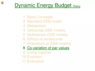
Dynamic Energy Budget theory. 1 Basic Concepts 2 Standard DEB model 3 Metabolism 4 Univariate DEB models 5 Multivariate DEB models 6 Effects of compounds 7 Extensions of DEB models 8 Co-variation of par values 9 Living together 10 Evolution 11 Evaluation.

E N D
Dynamic Energy Budget theory 1 Basic Concepts 2 Standard DEB model 3 Metabolism 4 Univariate DEB models 5 Multivariate DEB models 6 Effects of compounds 7 Extensions of DEB models 8 Co-variation of par values 9 Living together 10 Evolution 11 Evaluation
Scales of life 8a 30 Life span 10log a Volume 10log m3 earth 20 10 life on earth whale whale 0 bacterium ATP molecule -10 bacterium -20 water molecule -30
Selection for reproduction 8.1.1 Red Jungle fowl Indian River broiler White Leghorn
Dwarfing in Platyrrhini 8.1.2a 180 g Cebidae 130 g Saimiri 200-400 g Saguinus 400-535 g 480-700 g 400-450 g 780-1250 g 700-1000 g 3500 g Callitrix Callimico Cebuella Leontopithecus MYA Mico Aotus 24.8 20.2 Perelman et al 2011 Plos Genetics7, 3, e1001342 Cebus
Inter-species body size scaling 8.2 • parameter values tend to co-vary across species • parameters are either intensive or extensive • ratios of extensive parameters are intensive • maximum body length is • allocation fraction to growth + maint. (intensive) • volume-specific maintenance power (intensive) • surface area-specific assimilation power (extensive) • conclusion : (so are all extensive parameters) • write physiological property as function of parameters • (including maximum body weight) • evaluate this property as function of max body weight Kooijman 1986 Energy budgets can explain body size scaling relations J. Theor. Biol.121: 269-282
Primary parametersstandard DEB model 8.2.1 Kooijman 1986 J. Theor. Biol. 121: 269-282
Feeding strategies are adaptable 8.2.1b big prey filter feeding basking shark (Cetorhinus maximus) white shark, (Carcharodon carcharias) cookiecutter shark (Isistius brasiliensis) whale shark (Rhincodon typus)
Body weight 8.2.2 Body weight has contributions from structure and reserve If reserve allocated to reproduction hardly contributes:
West-Brown: scaling of respiration 8.2.2b Explanation: Minimizing of transportation costs in space-filling fractally branching tube systems results in ¾ - “law” West et al 1997 Science276: 122-126 Problems: • Protostomes have open circulation system, no tube system scaling of respiration also applies to protostomes • Flux in capillaries is much less than in big tubes, not equal • Transport rate must match peak metabolic requirements rather than standard • No differentiation between inter- and intra-specific scaling • Transport costs are tiny fraction of maintenance costs minimum argument is not convincing (nor demonstrated) • Scaling of respiration does not explain all other scaling “laws” nor “the growth curve” of demand systems
Banavar: scaling of respiration 8.2.2c Explanation: Dilution of biomass with transport material between maintenance-requiring nodes in efficient networks results in ¾ -”law”; Banavar et al 1999 Nature399: 130-132 Problems: • Transport rate must match peak metabolic requirements rather than standard • No differentiation between inter- and intra-specific scaling • criterion • Assumption about the scaling of mass involved in transport is not tested; tubing material does not dominate in whales • Efficiency criterion is anthropomorphic
Scaling of respiration 8.2.2d Respiration: contributions from growth and maintenance Weight: contributions from structure and reserve Kooijman 1986 J Theor Biol 121: 269-282
Metabolic rate 8.2.2e slope = 1 Log metabolic rate, w O2 consumption, l/h 2 curves fitted: endotherms 0.0226 L2 + 0.0185 L3 0.0516 L2.44 ectotherms slope = 2/3 unicellulars Log weight, g Length, cm Intra-species Inter-species (Daphnia pulex) Data: Richman 1958; curve fitted from DEB theory Data: Hemmingson 1969; curve fitted from DEB theory
Feeding rate 8.2.2f slope = 1 Filtration rate, l/h Mytilus edulis Data: Winter 1973 poikilothermic tetrapods Data: Farlow 1976 Length, cm Inter-species: JXm V Intra-species: JXm V2/3
Scaling relationships 8.2.2g log scaled initial reserve log scaled age at birth log zoom factor, z log zoom factor, z approximate slope at large zoom factor log scaled length at birth log zoom factor, z
Length at puberty 8.2.2h Clupoid fishes Sardinella + Engraulis * Centengraulis Stolephorus Clupea • Brevoortia ° Sprattus Sardinops Sardina Data from Blaxter & Hunter 1982 Length at first reproduction Lp ultimate lengthL
Von Bertalanffy growth rate 8.2.2i 25 °C TA = 7 kK 10log von Bert growth rate, a-1 10log ultimate length, mm 10log ultimate length, mm ↑ ↑ 0
Body temperature of Maiasaurs 8.2.2j • determine v Bert growth rate & max length • convert length to weight (shape) • obtain v Bert growth rate for that weight at 25 °C (inter-spec) • calculate ratio with observed v Bert growth rate • convert ratio to body temperature (inverse Arrhenius) • result: 37 °C length, cm age, a
Incubation time 8.2.2k European birds tube noses 10log incubation time, d 10log incubation time, d slope = 0.25 lb equal ° tube noses 10log egg weight, g 10log egg weight, g Data from Harrison 1975 Incubation time Egg weight
Gestation time 8.2.2l Mammals * Insectivora + Primates Edentata Lagomorpha Rodentia Carnivora Proboscidea Hyracoidea Perissodactyla Artiodactyla slope = 0.33 10log gestation time, d 10log adult weight, g Data from Millar 1981 Kooijman 1986 J Theor Biol 121: 269-282
Costs for movement 8.2.2m Movement costs per distance V2/3 Investment in movement V included in somatic maintenance Home range V1/3 Data: Fedak & Seeherman , 1979 Data: Beamish, 1978 slope = -1/3 slope = -1/3 Walking costs: 5.39 ml O2 cm-2 km-1 Swimming costs: 0.65 ml O2 cm-2 km-1
Ageing among species 8.2.2n Right whale slope 1/3, 1/5 Ricklefs & Finch 1995 • Conclusion for life span • hardly depends on max body size of ectotherms • increases with length in endotherms
Abundance 8.2.3 Data: Peters, 1983 feeding rate V food production constant Abundance V-1 Kooijman 1986 J Theor Biol 121: 269-282
1,1 compartment model 8.3.1 and Suppose while Kooijman et al 2004 Chemosphere 57: 745-753
Elimination rate & partition coeff 8.3.2 diffusivities low high 1 film 2 film log 10% saturation time log P01 log P01 Transition: film 1,1-compartment model Kooijman et al 2004 Chemosphere 57: 745-753
QSARs for tox parameters 8.3.4 Slope = -0.5 Slope = 1 Slope = -1 10log elim rate, d-1 10log kill rate, mM-1 d-1 10log NEC, mM 10log Pow 10log Pow 10log Pow Assumption: Each molecule has same effect Alkyl benzenes in Pimephales Data from Geiger et al 1990 • Hazard model for survival: • one compartment kinetics • hazard rate linear in internal concentration Kooijman et al 2004 Chemosphere 57: 745-753
QSARs for tox parameters 8.3.4a Slope = -0.5 Slope = 1 Slope = -1 10log elim rate, d-1 10log kill rate, mM-1 d-1 10log NEC, mM 10log Pow 10log Pow 10log Pow Benzenes, alifates, phenols in Pimephales Data from Mackay et al 1992, Hawker & Connell 1985 Assumption: Each molecule has same effect • Hazard model for survival: • one compartment kinetics • hazard rate linear in internal concentration Kooijman et al 2004 Chemosphere 57: 745-753
Covariation of tox parameters 8.3.4b Slope = -1 10log NEC, mM 10log killing rate, mM-1 d-1 Pimephales Data from Gerritsen 1997 Kooijman et al 2004 Chemosphere 57: 745-753
QSARs for LC50’s 8.3.4c 10log LC50.14d, M 10log Pow 10log Pow LC50.14d of chlorinated hydrocarbons for Poecilia. Data: Könemann, 1980
SimilaritiesQSAR body size scaling 8.4 1-compartment model: partition coefficient (= state) is ratio between uptake and elimination rate DEB-model: maximum length (= state) is ratio between assimilation and maintenance rate Parameters are constant for a system, but vary between systems in a way that follows from the model structure
InteractionsQSAR body size scaling 8.4a • uptake, elimination fluxes, food uptake surface area (intra-specifically) • elimination rate length-1 (exposure time should depend on size) • food uptake structural volume (inter-specifically) • dilution by growth affects toxicokinetics • max growth length2 (inter-specifically) • elimination via reproduction: max reprod mass flux length2 (inter-specifically) • chemical composition: reserve capacity length4 (inter-specifically) • in some taxa reserve are enriched in lipids • chemical transformation, excretion is coupled to metabolic rate • metabolic rate scales between length2 and length3 • juvenile period length, abundance length-3 , pop growth rate length-1 • links with risk assessment strategies
Dynamic Energy Budget theory 1 Basic Concepts 2 Standard DEB model 3 Metabolism 4 Univariate DEB models 5 Multivariate DEB models 6 Effects of compounds 7 Extensions of DEB models 8 Co-variation of par values 9 Living together 10 Evolution 11 Evaluation