Confocal Microscopy David Kelly November 2013

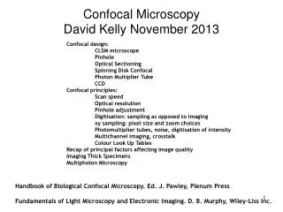
1. Confocal MicroscopyDavid Kelly November 2013 Confocal design: CLSM microscope Pinhole Optical Sectioning Spinning Disk Confocal Photon Multiplier Tube CCD Confocal principles: Scan speed Optical resolution Pinhole adjustment Digitisation: sampling as opposed to imaging xy sampling: pixel size and zoom choices Photomultiplier tubes, noise, digitisation of intensity Multichannel imaging, crosstalk Colour Look Up Tables Recap of principal factors affecting image quality Imaging Thick Specimens Multiphoton Microscopy Handbook of Biological Confocal Microscopy. Ed. J. Pawley, Plenum Press Fundamentals of Light Microscopy and Electronic Imaging. D. B. Murphy, Wiley-Liss Inc.

2. What to get out of this lecture Have an understanding of how a modern confocal microscope works Become familiar with the principal factors affecting image quality in the CLSM Begin to have an idea when and how to manipulate these factors for your purposes This often means knowing when and where to make compromises (e.g. light collection versus spatial resolution)

3. Benefits of Confocal Microscopy Reduced blurring of the image from light scattering Increased effective resolution Improved signal to noise ratio Clear examination of thick specimens Z-axis scanning Depth perception in Z-sectioned images Magnification can be adjusted electronically

4. Confocal Design

5. CLSM microscope antivibration table

6. Confocal principle

7. Conjugate plane The Pinhole y z y x x

8. The Pinhole Pinhole

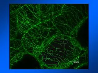
9. Optical sectioning 1 mm

10. Laser scanning Photomultiplier tube Computer

11. Laser scanning xy scanning y z y y x x x single section z series z z z x y y x x xz scanning

12. Confocal Principles

13. Scan speed: t resolution On modern confocals this is measured in Hz usually from 1-1400Hz Decreasing scan speed- more light collected (dwell time increased) more chance of photobleaching and phototoxicity limits temporal resolution Increasing scan speed- has opposite effect but often results in poor image quality Note: Some types of confocal specifically optimised for fast scanning. Eg spinning disk, line scanner and resonant scanner

14. Pinhole adjustment Airy disc 0.5 Maximum optical sectioning and resolution. Discard much in-focus light • xy resolution approaches that of conventional microscopy, but still retain good rejection of out-of-focus information. Still lose some in-focus photons. >1 Maximise light collected. But this mostly comes from adjacent out-of-focus planes - lose z resolution. xy resolution not badly affected Open pinhole z z Close pinhole y y x x

15. Confocal Pinhole

16. z = 2 z = 4 z = 0 210 nm 60 nm z = 6 z = 8 Fluotar 20x/0.5 Zoom = 3 Pinhole = 0.7

17. z = 2 z = 4 z = 0 210 nm 60 nm z = 6 z = 8 Fluotar 20x/0.5 Zoom = 3 Pinhole = 3.0

18. Pinhole Summary • In practise, pinhole size is mainly used to control optical section thickness other than to achieve highest lateral or Z-resolution • Occasionally, pinhole size can be used to adjust amount of photon received by PMT to change the signal intensity and increase SNR. In addition to the "optimal" 1 AU, Pinhole  1-3 AU is the range of choice. Bigger pinhole give you stronger signal but with the compromised confocal effects.

19. Sampling Scanning involves digitisation in x, y, z, intensity, and t Resolution is affected by sampling during the digitisation process 0 0 0 0 0 0 0 0 0 0 0 0 0 0 0 0 22 45 66 11 0 0 0 0 0 0 0 0 0 0 0 0 0 0 0 0 0 0 0 0 0 0 0 0 0 0 65 12 0 0 0 0 0 0 0 0 0 0 0 0 99 0 0 0 0 pixels (voxels) 0 0 0 0 0 0 0 7 0 0 0 0 0 0 0 6 5 0 0 0 2 8 21 5 2 0 0 0 0 3 0 0 0 0 0 0 0 0 0 0 0 0 0 0 0 0 0 0 0 0 0 0

20. Pixel choices 512x512 1024x1024 2048x2048 —250 kbyte (1 channel) —3 Mbyte (3 channel) More pixels— smoother looking image - more xy information more light exposure of specimen larger file size slower imaging (less temporal resolution)

21. Digitisation can lose information Correct choice of pixel size can minimise this intensity scan line

22. Specimen Large pixels Small pixels, lucky alignment Small pixels, unlucky alignment Very small pixels Pixel undersampling

23. Nyquist sampling (xy) Optimum pixel size for sampling the image is at least 1/2 spatial resolution 100x, 1.35 NA, 520 nm (blue-green) Spatial resolution = 0.15 mm Required pixel size = 0.075 mm Actual pixel size at 512x512 is usually too large (will be shown on screen or calculate from field size/pixel number) How to adjust to meet Nyquist criteria? Use higher pixel number (e.g. 1024x1024 2048x2048) or use a zoom factor…

24. Zooming Using the same scanning raster, speed, illumination on a smaller area of the field of view May ideally need 2–5x zoom to satisfy the Nyquist criteria.

25. Nyquist Sampling Equation i) 0.4 x wavelength/NA = Resolvable Distance ii) 2 pixels is smallest optically resolvable distance iii) Resolvable Distance/2 = smallest resolvable point

26. Nyquist Sampling Example • X10 Objective with 0.3 NA using GFP • 0.4 x 520 = 693nm 0.3 693 = 346.6nm smallest resolvable distance 2 • Scan Size = 1500µm • Box Size = 1024 pixels • 1500 = 1464nm 1024 1464 = 4.2 zoom for nyquist in xy 346.6 Or a box size large enough to produce a pixel size of 346.6

27. Nyquist sampling and z series What distance between z steps? Optimum z step for sampling the image is 1/2 the axial resolution For high NA lens of 0.3 mm z resolution, optimum z stepping is 0.1-0.2 mm (assuming optimum pinhole size, etc). In practice, this is often too many for a very thick specimen. 0.5-1 mm is often fine. Especially if pinhole opened. z y x

28. Over- and undersampling Oversampling (pixels small compared with optical resolution) Image smoother and withstands manipulation better Specimen needlessly exposed to laser light Image area needlessly restricted File size needlessly large Undersampling (pixels large compared with optical resolution) Degraded spatial resolution Photobleaching reduced Image artefacts (blindspots, aliasing) “If you must sample below the Nyquist limit, then spoil the resolution [to match better the pixel size]!” ie. Open the pinhole.

29. Digitisation of PMT voltage Voltage is sampled at regular intervals and converted into a digital pixel intensity value by the analogue-digital converter (ADC) 12 bit 1 bit: 2 levels (black + white) 7 3 bit 8 levels of brightness Level 3 bit 0 x (Eye is a 6 bit device (~50 levels of brightness))

30. Noise Noise: any variability in measurement that is not due to signal changes S/N ratio determines the lower limit of the ability to distinguish true changes in the measurement (dynamic range) Photon sampling variability (shot noise): Statistical fluctuations in photons hitting PMT. Electronic noise: Variability in PMT generated current. These things are exacerbated at high gain settings Reduce noise by sampling more photons: Reducing scan rate (increasing pixel dwell time), or opening pinhole. Frame averaging Noise is reduced (dynamic range increased) with square root of number of frames Sample exposure to light is increased

31. 1 scan 16 scans Medium gain Laser 488nm 80% PMT 800V High gain Laser 488nm 10% PMT 1000V Apo 63x lens

32. Digitisation of intensity Normally 8 bit (256 brightness levels) Extended dynamics 12 bit (4095 brightness levels) But useful dynamic range is degraded by noise Why need so many bits? 1. Spare dynamic range for exploring intensity details during image processing 2. Probably helps to smooth out noise problems (e.g. capture in 12 bit and save in 8 bit) Quantitation/physiology

33. Multi-channel imaging

34. Multi-channel imaging Use a fluorochrome combination Multiple laser lines and PMTs Complicated filter sets needed to separate light Alternatives: AOTF, AOBS, spectrophotometric detection 488, 568 >550 PMT2 Dichroic mirrors or AOBS <550 bleedthrough PMT1

35. Crosstalk FITC = fluorescein isothiocyanate TRITC = tetramethyl rhodamine isothiocyanate FITC TRITC Green channel Red channel Usually overlap of emission spectra from L to R

36. Crosstalk How to test: Turn off laser line for the ‘LH’ fluorochrome How to reduce: Use better separated fluorochromes e.g. FITC + Texas Red versus FITC + TRITC Put the weak signal in the ‘LH’ channel Sequential imaging rather than simultaneous imaging

37. Preventing cross-talk FITC TRITC FITC Texas Red

38. 4 principal factors for image quality Spatial resolution Ultimately set by the optics, but can be limited by digitisation (therefore affected by image size and zoom). Affected by pinhole: super-resolution (1.4x) is possible at small pinholes Intensity resolution Ultimately set by detector, but limited by digitisation and low photon sampling. Aim to fill whole dynamic range with image information. Signal-to-noise ratio Degree of visibility of image over background noise, given variability in system. Temporal resolution Depends on raster scan rate (+averaging). 512x512 at 2/s. Imaging depends on compromising between these factors, e.g. you might want to optimise resolution of light intensity at expense of spatial or temporal resolution.

39. Colour Look UpTables Which colours to use? You’re not restricted to the ‘true’ colour of the fluorochrome Colour look-up table

40. Colour LUT Grey is bestRed is really bad

41. Imaging Thick Specimens

42. The Problem

43. Defocus 1µm

44. Background & Scattering Confocal Widefield

45. Red Green Blue Aberrations Blue Green Red Lateral Chromatic Aberration Axial Chromatic Aberration

46. Aberrations Chromatic No-Aberration Green-Red Chromatic Aberration

47. Aberrations Spherical Aberration 20-40µm

48. Aberrations nls GFP: ex 476; em 530+/-15 Spherical Aberration on aconfocal XZ 75 um XY coverslip 0 um 100 um 100 um

49. S* S* S S 2-Photon 1-photon absorption 2-photon absorption Fluorescence Fluorescence

50. 2-Photon Single Photon 2 photon