Download

1 / 39
400 likes | 619 Vues
Nonconvex Rigid Bodies with Stacking. Eran Guendelman Robert Bridson Ron Fedkiw Stanford University. Paper Overview. Goal: Plausible simulation of a large number of nonconvex rigid bodies. Handle collision, contact, friction, stacking. Main Contributions. A new time stepping scheme.

E N D
Nonconvex Rigid Bodies with Stacking Eran Guendelman Robert Bridson Ron Fedkiw Stanford University
Paper Overview Goal: • Plausible simulation of a large number of nonconvex rigid bodies. • Handle collision, contact, friction, stacking.
Main Contributions • A new time stepping scheme. • A “shock propagation” technique for stacks.
Geometric Representation • A dual representation. • Explicit: Triangulated surface. • Supplies point samples on surface. • Implicit: Signed distance function Φ. • Φ distance to surface, Φ< 0inside, Φ> 0 outside. • Stored on a uniform or octree grid. • Constant time inside/outside test. • Normal = Φ (defined throughout space).
Time Stepping: Traditional Approach • Traditional time stepping simulation loop: • Update position and velocity. • Process collision. • Process contact.
Problem With Traditional Approach • Problem: e.g. Block sliding down inclined plane. • Initially sliding down. • Update position and velocity interpenetrating plane. • Process collision velocity reflected. • No contact to process. • Next iteration object bounces.
Fixing Problem • Velocity threshold. • e.g. [Mirtich & Canny ’95 – 2 papers] • Process as contact if speed below threshold. • Our approach doesn’t require such threshold.
Time Stepping:Our Approach • A new ordering of the simulation loop: • Process collision. • Update velocity. • Process contact. • Update position. • Some justification: • Velocity update integrates forces and contact processing resolves forces. • Recall traditional approach: • Update pos & vel. • Process collision. • Process contact.
Inclined Plane Revisited • Using our approach. • No collision to process. • Update velocity block gains downward velocity. • Process contact stops normal motion. • Update position slides down with no bounce.
Time Stepping Comparison • Errors accentuated: • Perfectly elastic collisions (ε=1). • We don’t rewind to collision time. • Impulses applied sequentially at point samples.
Accuracy Decelerating down inclined plane
Accuracy Accelerating down inclined plane
Simulation Step • Choose sufficiently small time step ∆t. • Advance bodies using time stepping scheme. • Use forward Euler for position and velocity update. • Doesn’t guarantee non-interpenetration, but achieves good results. • Experimented with “pushing out” to reduce penetration as in [Baraff ‘95].
Interference Detection • We don’t rewind to collision time. • Find all penetrating vertices. • Use implicit surface inside/outside test. • Optionally compute edge-face intersections. • Accelerations: • Uniform spatial partition. • Bounding boxes.
Impulse • Impulses are used for collision and contact. • Collision parameters: ε and μ. • Collision normal = Φ. • Use Coulomb friction model: • Compute impulse to stop tangential motion. • If outside friction cone, find kinetic friction impulse. • Similar to [Hahn ‘88; Moore & Wilhelms ‘88]. • Rolling and spinning friction.
Collision Processing • Detect and resolve collisions during time step. • One approach: Process in chronological order. • Computationally expensive for scenes with frequent collisions. • Approach we use: Process all at end of step. • Gives plausible results. • Don’t need to rewind to exact time of collision.
Collision Processing: Algorithm Overview • Compute candidate positions of bodies. • For each intersecting pair of bodies: • Determine interpenetrating points. • Sort points by penetration depth (deepest first). • For each point in order: • Apply frictional impulse (unless bodies receding).
Collision Processing:Algorithm Overview • Repeat above a number of times. • Resolving one collision might create new ones. • Applies series of impulses rather than simultaneously resolving all collisions.
Contact Processing • Determine contacts and prevent penetration. • Approaches: • Simultaneously solve for all contact forces. e.g.[Baraff ‘94] • Penalty method (repulsion forces). e.g.[Moore & Wilhelms ‘88] • Approach we use: • Approximate continuous contact by a series of inelastic impulses. e.g. [Mirtich & Canny ‘95] • Algorithm similar to collision processing (with ε=0), but modified for improved accuracy.
Improving Accuracy • Gradually slow down bodies. • Transition impulses from ε=-1 to ε=0. • -1<ε<0: Slows normal approach velocity. • Use more (smaller) impulses for contact. • Compute impulses in old position. • Still use candidate position to find contact points. OLD CANDIDATE
Contact Processing: Problem With Stacks • Problem with stacks: Need many iterations.
Computing Stack Ordering • Order bodies in stacks into increasing levels: • Compute directed graph of “resting on” relation. • Group together cycles (get a DAG). • Find levels consistent with DAG.
Shock Propagation • Process contact bottom-up. • After processing a level, set to infinite mass (but not static).
Combining Contact and Shock Propagation • Run a number of regular contact iterations. • Without setting levels to infinite mass. • Transmits weight through stack. • Run a single iteration of shock propagation. • Get good behavior without requiring many iterations.
Summary • Dual representation of geometry. • Impulse-based simulator. • New time stepping approach eliminates need for a velocity threshold. • Shock propagation shocks the stack into a reasonable configuration without requiring many contact iterations.