Implementation and Design of Realistic Module for MuCh Software in CBM @ SIS100
This document outlines the implementation of a realistic module design for the MuCh software utilized in the CBM experiment at SIS100. Key aspects include segmentation algorithms, digitization algorithms, and hit finding algorithms. The design features simple geometries for stations, simulated as 3mm disks of argon gas, with overlaps in active volumes for efficient detection. Major focus areas include support structures, estimated dimensions, and the challenge of handling large parameter files. The overall goal is to improve readability and flexibility in module design and simulation processes.

Implementation and Design of Realistic Module for MuCh Software in CBM @ SIS100
E N D
Presentation Transcript
Status of MuCh software • Outline • Implementation of realistic module design • Segmentation algorithms • Digitization algorithm • Hit finding algorithm • Visual display for MUCH Evgeny Kryshen (PNPI) Mikhail Ryzhinskiy (PNPI & SPbSPU)
Old geometry • Stations are simulated as simple shapes – 3mm disks filled with argon gas • Distances between layers and absorbers are not realistic (too small) • No support structures, no module design • Parameter files are huge, full of irrelevant numbers, hardly readable, not flexible CBM @ SIS100, 21 May 2009
Module design in ALICE CBM @ SIS100, 21 May 2009
Schematic layout of GEM module Pads Readout electronics PCB Argon Spacer Support structure Fasteners GEM foils CBM @ SIS100, 21 May 2009
Implementation of module design Front side Back side Overlap • Layers: • Modules are arranged in rows on both sides of each layer • There is an overlap of active volumes to avoid dead zones in y direction CBM @ SIS100, 21 May 2009
Support structures and modules • Support structures: • Each support structure is composed of two parts to assure easy installation around the pipe • Estimated thickness ~ 1.5 cm • Material: carbon plastics (ρ = 0.1 ρC) • Implemented as composite shapes in cbmroot • Module: • Module size is mostly restricted by the GEM foil production technology • Active volume: 256 x 256 mm x 3 mm, argon • Spacers: 5 cm in y, 0.5 cm in x; material: noryl, implemented as composite shapes • Active volume implemented as TGeoBox for simple modules and as composite shapes for modules with a hole X spacers Active volume Y spacers CBM @ SIS100, 21 May 2009
Detailed geometry: general view Module design Simple design Straw design • Two layers at each station • Three layers at the last trigger station • Modules are automatically located on the surface of support structures • Cables, gas tubes, PCBs and front-end electronics are neglected at the moment CBM @ SIS100, 21 May 2009
Geometry input file: much_standard_straws.geo # General information MuchCave Zin position [cm] : 105 Acceptance tangent min : 0.1 Acceptance tangent max : 0.5 Number of absorbers : 6 Number of stations : 6 # Absorber specification Absorber Zin position [cm] : 0 40 80 120 170 225 Absorber thickness [cm] : 20 20 20 30 35 100 Absorber material : I I I I I I # Station specification Station Zceneter [cm] : 30 70 110 160 215 340 Number of layers : 2 2 2 3 3 3 Detector type : 1 1 1 2 2 2 Distance between layers [cm]: 10 10 10 7 7 7 Support thickness [cm] : 1.5 1.5 1.5 0.0 0.0 0.0 Use module design (0/1) : 1 1 1 0 0 0 # GEM module specification (type 1) Active volume lx [cm] : 25.6 Active volume ly [cm] : 25.6 Active volume lz [cm] : 0.3 Spacer lx [cm] : 0.5 Spacer ly [cm] : 5 Overlap along y axis [cm] : 2 # Straw module specification (type 2) Straw thickness [cm] : 0.4 CBM @ SIS100, 21 May 2009
Class hierarchy CbmMuchGeoScheme CbmMuchStation CbmMuchLayer CbmMuchLayerSide CbmMuchModule CbmMuchSector CbmMuchPad CBM @ SIS100, 21 May 2009
Automatic segmentation: algorithm y Hit density vs R x // Set minimum allowed resolution for each station Double_t sigmaXmin[] = {0.04, 0.04, 0.04, 0.04, 0.04, 0.04}; Double_t sigmaYmin[] = {0.04, 0.04, 0.04, 0.04, 0.04, 0.04}; seg->SetSigmaMin(sigmaXmin, sigmaYmin); // Set maximum allowed resolution for each station Double_t sigmaXmax[] = {0.32, 0.32, 0.32, 0.32, 0.32, 0.32}; Double_t sigmaYmax[] = {0.32, 0.32, 0.32, 0.32, 0.32, 0.32}; seg->SetSigmaMax(sigmaXmax, sigmaYmax); // Set maximum occupancy for each station Double_t occupancyMax[] = {0.05, 0.05, 0.05, 0.05, 0.05, 0.05}; seg->SetOccupancyMax(occupancyMax); CBM @ SIS100, 21 May 2009
Automatic segmentation: results Simple design Module design • Sector sizes at the first station are mostly determined by occupancy restrictions • Starting from the 3rd station sector sizes are determined by the required resolution • The smallest pad size in the default setup is ~2 mm (resolution ~ 600 μm). CBM @ SIS100, 21 May 2009
New flexible (manual) segmentation Module design Simple design // Number of regions for each station Int_t nRegions[] = {5, 3, 1, 1, 1, 1}; seg->SetNRegions(nRegions); // Set region radii for each station Double_t st0_rad[] = {13.99, 19.39, 24.41, 31.51, 64.76}; seg->SetRegionRadii(0, st0_rad); … // Set minimum pad size/resolution in the center region for each station Double_t padLx[] = {0.1386, 0.4, 0.8, 0.8 ,0.8, 0.8}; seg->SetMinPadLx(padLx); Developed by M. Ryzhinskiy CBM @ SIS100, 21 May 2009
Digitization algorithm Primary electrons: Number of primary electrons is generated according to Landau distribution (MPV and sigma taken from HEED) MPV and sigma are calculated for electrons, muons and protons. For other particle types we use mass scaling. Secondary electrons: Exponential gas gain distribution with mean value of 104 sec. electrons/prim. electron Sec. electrons are projected on pads in a circle with a given spot radius (0.3 mm for MM, 1.5 mm for GEM) Charge thresholds: Maximal charge for muon track: 4x10⁵ electrons/pad For 256 channel ADC one has 1.5x10³ electrons/channel Minimum charge threshold: 3 channels Factors not taken into account: Transverse diffusion of primary electrons is not accounted for Cluster nature of primary electrons CBM @ SIS100, 21 May 2009
Charge distribution Mean charge: 3.6∙105 (In average 36 primary electrons) • Factors contributing to the charge dispersion: • Particle type • Particle energy • Track length variation • Number of “primary” electrons generated according to Landau distribution with a given MPV and sigma (dependent on Particle energy and type) • Gas gain fluctuations in accordance with exponential distribution with mean value of 10000 CBM @ SIS100, 21 May 2009
Energy dependence of the charge X axis – decimal logarithm of track energy measured in MeV Y axis – charge generated by track (number of secondary electrons) The sharp cut-off at Log E equal to 0 ( or equivalently 1 MeV) is due to the geant3 minimum energy cut CBM @ SIS100, 21 May 2009
Energy dependence of the charge Charge vs energy distributions for different particle types: CBM @ SIS100, 21 May 2009 • Solid lines correspond to MPV energy dependencies built in the simulation (MPV curve is proportional to Bethe-Bloch in the first approximation) • These plots demonstrate the consistency of the simulation • Electrons are most sensitive to 1 MeV cut-off • Detailed studies of the electron cut-off dependency are desired
Charge vs. track length • Sensitive gap of the detectors is 3 mm • Difference in the track length is caused by the track slope • The large track length is usually caused by secondaries • Track lengths smaller than 3 mm are due to edge effects • Mean length for electrons: 4.5 mm • Mean length for protons: 3.5 mm CBM @ SIS100, 21 May 2009
Illustration of fired pads CBM @ SIS100, 21 May 2009
Cluster deconvolution Q Qmax Qthr Primary cluster Hit coordinates: Hit errors: Qthr(Qmax) = 0.1Qmax pads CBM @ SIS100, 21 May 2009
Cluster statistics • Mean number of generated MC points contributing to one cluster: 1.16 • Mean number of fired pads in one cluster: 2.33 • Mean number of reconstructed hits produced in one cluster: 1.02 CBM @ SIS100, 21 May 2009
Hit finding results inactive pads fired pads traces from MC tracks reconstructed hits – 3000 MC points/event CBM @ SIS100, 21 May 2009
Fake hits 0.3% Fake hits – number of reconstructed hits is larger than the number of tracks which formed the cluster CBM @ SIS100, 21 May 2009
Lost hits Lost hits – number of reconstructed hits is less than the number of tracks which formed the cluster 10.1% Conclusion: the naive hit finding algorithm should be improved CBM @ SIS100, 21 May 2009
Visual Event Display: Layer view Layer view functionality: • Switch between stations and layers • Info on stations • Zoom • Show info on hits, points and sectors • Switch off sectors, modules, layer sides, hits and points • Select particles with required PDG code and mothers • Browse events • Clickable sectors producing zoomed module views CBM @ SIS100, 21 May 2009
Visual Event Display: Module View Zoomed module view Fired pads are marked with blue gradient colors reflecting the accumulated charge Found hits are marked with black markers CBM @ SIS100, 21 May 2009
Visual Event Display: Cluster View Cluster view can be opened by clicking on a cluster in a module frame. It is aimed to help in optimization of hit finding algorithms. CBM @ SIS100, 21 May 2009
Future plans • Implementation of straw digitization and hit finding • Implementation of “mixed” stations with modules of different types • Optimization of the software with respect to tracking requirements • Optimization of digitization parameters and detector layout • Development of advanced cluster deconvolution algorithm • Further development of visualizer CBM @ SIS100, 21 May 2009