Reynolds-Averaged Navier -Stokes Equations -- RANS
Reynolds-Averaged Navier -Stokes Equations -- RANS. 4 equations; 7 unknowns. Similar situation as when we went from Cauchy’s eq to N-S eq. A j = eddy viscosity. [m 2 /s]. Turbulence Closure. Turbulent Kinetic Energy (TKE). Total flow = Mean plus turbulent parts =. Same for a scalar:.

Reynolds-Averaged Navier -Stokes Equations -- RANS
E N D
Presentation Transcript
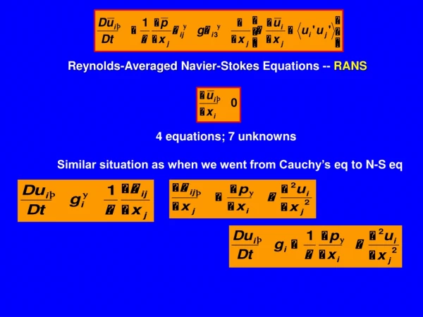
Reynolds-Averaged Navier-Stokes Equations -- RANS 4 equations; 7 unknowns Similar situation as when we went from Cauchy’s eq to N-S eq
Aj= eddy viscosity [m2/s] Turbulence Closure
Turbulent Kinetic Energy (TKE) Total flow = Mean plus turbulent parts = Same for a scalar: Start with momentum equation (balance) for total flow: and subtract momentum equation for mean flow: yields the momentum equation for turbulent flow: An equation to describe TKE is obtained by: multiplying the momentum equation for turbulent flow times the turbulent flow itself (scalar product) and then do ensemble averages
Multiplying turbulent flow momentum equation times uiand dropping the primes (all lower case letters are turbulent or fluctuating variables) fluctuating strain rate Turbulent Kinetic Energy (TKE) Equation Total changes of TKE Transport of TKE Shear Production Buoyancy Production Viscous Dissipation Transport of TKE. Has a flux divergence form and represents spatial transport of TKE. The first two terms are transport of turbulence by turbulence itself: pressure fluctuations (waves) and turbulent transport by eddies; the third term is viscous transport
interaction of Reynolds stresses with mean shear; represents gain of TKE represents gain or loss of TKE, depending on covariance of density and w fluctuations represents loss of TKE http://apollo.lsc.vsc.edu/classes/met455/notes/section4/1.html
In many ocean applications, the TKE balance is approximated as:
Turbulence Production and Cascade Injective range -- large scales where forcing injects the energy Inertial range -- where the time required for energy transfer is shorter than the dissipative time and the energy is thus conserved and transported to smaller scales. Dissipative range -- where the energy dissipation overcomes the transfer and the cascade is stopped. Inertial range http://math.unice.fr/~musacchi/tesi/node9.html “Big whorls have little whorls That feed on their velocity; And little whorls have lesser whorls, And so on to viscosity.” (Lewis F Richardson, 1920)
The rate of energy transfer to smaller scales can be estimated from scaling: u velocity of the eddies containing energy l is the length scale of those eddies u2 kinetic energy of eddies l/ u turnover time u2/ (l /u )rate of energy transfer = u3 / l ~ At any intermediate scale l, But at the smallest scales LK, Kolmogorov length scale so that Typically, The largest scales of turbulent motion (energy containing scales) are set by geometry: - depth of channel - distance from boundary
Turbulence Cascade has a well defined structure – Kolmogorov’sK-5/3 law Spectral power S = sin(2 π t /30) S T = 30 s Time (secs) Spectral Amp (e.g. m2/Hz) Frequency (Hertz)
S = sin(2 π t /30) + sin(2 π t /12) S Time (secs) Spectral Amp (e.g. m2/Hz) Frequency (Hertz)
S = sin(2 π t /30) + sin(2 π t /12) + sin(2 π t /43) S Time (secs) Spectral Amp (e.g. m2/Hz) Frequency (Hertz)
S (m3 s-2) Wave number K (m-1)
P equilibrium range inertial dissipating range Kolmogorov’s K-5/3 law P & small in inertial range -- vortex stretching (Monismith’s Lectures)
Data from Ichetucknee River -5/3 Hour from 00:00 on
Kolmogorov’s K-5/3law -- one of the most important results of turbulence theory (Monismith’s Lectures)