Introduction to Computer Vision: Course Structure, Topics, and Applications
This course presents a comprehensive overview of Computer Vision, exploring topics such as image processing, 3D reconstruction, and geometric modeling. Classes are scheduled for Tuesdays and Thursdays, including four labs and a mix of assessments accounting for 30% labs, 30% mid-term, and 40% final exam. Key applications in fields like robotics, medical imaging, and security will be discussed, alongside fundamental mathematical tools and image quality principles. Join us for an engaging journey into the intersection of vision, graphics, and image-based modeling.

Introduction to Computer Vision: Course Structure, Topics, and Applications
E N D
Presentation Transcript
Course organisation • Lectures on Tuesday and Thursday • 4 labs (or mini-projects) • Mid-term and final • 30% labs+30% midterm+40%final
What is Computer Vision about? These fields are all closely related to 2d images, but different: Image processing: 2D images 2D images, well-defined pb. Computer vision: 2D images 3D reconstruction, hard ill-posed inverse pb. Computer graphics: 3D 2D, well-posed forward pb (+analysis & Interpretation)
What are applications? • modeling for graphics • visualization • photo/video manipulation and editing • robot navigation • autonomous vehicules • guiding tools for blind • security and monitoring • object/face recognition, OCR • medical applications • visual communication • digital libraries • …
What am I doing? Some examples
Overview • Introduction • intersection of vision, graphics and image-based modeling and rendring • some basic mathematical tools (linear algebra, homogeneous coordinates, and optimisation) • Modeling • Digital photography • Basic radiometry • Geometric modeling of camera • Camera calibration and pose estimation • Image features • Filtering • Edge detection, polygonal approximation • Points of interest detection • 3D reconstruction by multiple views: stereovision • Epipolar geometry • Computing correspondences • 3D reconstruction
On-line computer vision courses http://www.dai.ed.ac.uk/CVonline/
Digital Images World Camera Digitizer Digital Image geometry Image Formation: (i) What determines where the image of a 3D point appears on the 2D image? (ii) What determines how bright that image point is? (iii) How is a digital image represented? (iv) Some simple operations on 2D images? today Reflectance, radiometry
What is a digital image? Black/white = grayscale image Pixel: picture element Typically: 0 = black 255 = white x = 58 59 60 61 62 63 64 65 66 67 68 69 70 71 72 41 42 43 44 45 46 47 48 49 50 51 52 53 54 55 210 209 204 202 197 247 143 71 64 80 84 54 54 57 58 206 196 203 197 195 210 207 56 63 58 53 53 61 62 51 201 207 192 201 198 213 156 69 65 57 55 52 53 60 50 216 206 211 193 202 207 208 57 69 60 55 77 49 62 61 221 206 211 194 196 197 220 56 63 60 55 46 97 58 106 209 214 224 199 194 193 204 173 64 60 59 51 62 56 48 204 212 213 208 191 190 191 214 60 62 66 76 51 49 55 214 215 215 207 208 180 172 188 69 72 55 49 56 52 56 209 205 214 205 204 196 187 196 86 62 66 87 57 60 48 208 209 205 203 202 186 174 185 149 71 63 55 55 45 56 207 210 211 199 217 194 183 177 209 90 62 64 52 93 52 208 205 209 209 197 194 183 187 187 239 58 68 61 51 56 204 206 203 209 195 203 188 185 183 221 75 61 58 60 60 200 203 199 236 188 197 183 190 183 196 122 63 58 64 66 205 210 202 203 199 197 196 181 173 186 105 62 57 64 63 y =
Three types of images: • Gray-scale images I(x,y) [0..255] • Binary images I(x,y) {0 , 1} • Color images IR(x,y) IG(x,y) IB(x,y)
Image qualtiy: • resolution (size, #pixels, aspect ratio) • color depth • compression
Resolution: This graphic shows the relative sizes of a frame of 35mm film (red), the D60 image sensor (yellow), and a 1/1.8 CCD used in another digital camera (blue).
Image Width x height Aspect Ratio 35 mm film 36 x 24 mm 1.50 Display monitor 1024 x 768 1.33 Nikon Coolpix 990 2048 x 1536 1.33 Photo paper 4 x 6 inches 1.50 Photo paper 8 x 10 inches 1.25 Cannon EOS D60 3072 x 2048 1.5 HDTV 16 x 9 1.80 Aspect ratio:
Effects of down-sampling (reducing number of pixels): 4 x 4 32 x 32 128 x 128
Color depth: #bit for each pixel in each channel Resolution isn't the only factor, equally important is color depth, pixel-depth, or bit-depth.
Effects of reducing number of bits for each pixel: 2 gray levels (1 bit/pixel) BINARY IMAGE 256 gray levels (8 bits/pixel) 8 gray levels (3 bits/pixel)
Compression: A less compressed one A heavily compressed image
Image processing 1) Basic (global and nonlinear) operators 2) Spatial Domain 3) Frequency Domain - Histogram equalization - Gamma correction etc... later
Image histograme: A histogram is a graph that shows how the 256 possible levels of brightness are distributed in the image.
Continuous probability density function: Occurrence (# of pixels) Gray Level Histogram = The gray-level distribution: H(k) = #pixels with gray-level k Normalized histogram: Hnorm(k)=H(k)/N (N = # pixels in the image)
PI(k) 1 k PI(k) 1 0.5 k PI(k) 0.1 k
PI(k) 0.1 k 0.5 PI(k) 0.1 k Histogram Stretching
k k Histogram Equalization
Original Equalized
Gamma correction: Gamma correction controls the overall brightness of an image. Images which are not properly corrected can look either bleached out, or too dark. Trying to reproduce colors accurately also requires some knowledge of gamma. Varying the amount of gamma correction changes not only the brightness, but also the ratios of red to green to blue.
Sample Input to Monitor Output from Monitor Graph of Output L = V ^ 2.5 Graph of Input Correction L' = L ^ (1/2.5)