Download
1 / 35
350 likes | 364 Vues
Explore the innovative magnetic particle tracking system for studying fluidized beds. Acquire statistically significant data and develop correlations for fast-running models. Understand the detailed dynamics and behavior of solids in fluidized beds. Improve accuracy of fluidized bed process models.

E N D
Magnetic Particle Tracking in Spoutingand Bubbling Fluidized Beds Jack Halow Separation Design Group Stuart Daw Oak Ridge National Laboratory Presented at the 2012 Fall National Meeting of the American Institute of Chemical Engineers October 16-21, 2011 Pittsburgh, Pennsylvania
Objectives • Develop and demonstrate a unique experimental magnetic particle tracking system (MPTS) for studying solids mixing and dynamics in fluidized beds • Apply MPTS to develop statistically significant measures that characterize fluidized solids behavior • Develop correlations to develop fast running models of fluidized bed processes • Acquire data sets that can be used for validation of first principles and two phases and process models.
The magnetic particle tracking system • Tracer particles are constructed over a tiny neodymium magnet core • Magnet is Imbedded in a bead, foamed or coated • Tracer particles used are >1 mm diameter, 0.4-7 g/cc • Single tracer particles are injected into bed • Magnetic field signals recorded for analysis • Special algorithms deconvolute signals to give 3D trajectory data
Four inch bed with current MPTS setup • Probes aligned North, South, East, West • Helmholtz coils modify earth’s magnetic field in bed • Non-metallic bed and supports
MTPS Current Capabilities • Beds up to 10 cm in diameter • Sampling rates up to 200 hertz • Runs times to 10 minutes • Sensitivity <0.5 milligauss equivalent to ~20 cm • Temperatures to 200-300 Centigrade possible • Applications to fluid beds, granular flow or fluid flow system • Tracer sizes > ~ 1 mm and densities > 0.4 g/cc • Trade off sometimes required between parameters
Information we get from MPTS • 3D trajectory data • Visualize tracer motion • Position versus time graphs (i.e. Z or R vs time) • Short time 3D vector plots: particular types of events • 2D projections • Visualize average location • “Dot cloud” plots of data • 3D clouds or 2D slices • Quantify spatial information • Frequency distributions • Fit to statistical models for use in process model • Quantify temporal information • Autocorrelation analysis to yield characteristic times • FFT for highly periodic processes
Experiments I’ll discuss • Test conditions • 5.5 cm diameter bed • Porous plate distributor • 175 to 250 micron glass beads • 2.5 Umf (~15 cm/sec) • Slumped bed L/D =1 • 0.76 g/cc 4 mm tracer • Sampling rate was 100 Hertz • Run time was 5 minutes • 5 replicate tests performed • Data representations and analysis
3D views of three tests • “Dot clouds” give average temporal representations • But replicates not directly comparable Top View Side View
Statistical comparisons are better • Direct one to one comparisons not viable • Overall conditions same but detailed dynamics depend on detailed local initial conditions which are never identical • Spatial statistical comparison • Compare frequency distributions - probability of spatial location • Temporal statistical comparison • Compare autocorrelation curves at various time lags - characteristic cycle times
Spatial comparison: frequency plots • Divide vertical height into 40 bins • Place each measured z into a bin and count up each bin • Calculate normalized frequency for each bin
Length of test is important • Compares full tests and segments of a test • Agreement deteriorates with shorter times • Need adequate run times to characterize bed 300 sec 50 sec 25 sec
Temporal comparison • Autocorrelation function • Compares times series to itself as it’s shifted in time • Periodicity shows up as peaks in the correlation coefficient ~0.8 sec cycle time
Radial position at various levels • Dots in ring at higher bed levels • Concentrated in center lower in bed
Radial Frequency Distributions • For each of the six levels: • Radial position sorted into 7 even radius bins • Points counted and normalized for each bin
Radial position autocorrelation • Doesn’t show significant correlation • Radial motion essentially random • Bubble position radially random
Velocities show bubble events • 5 second segment • X & Y spikes indicate rapid lateral motion from bubbles • X & Y motion coupled with vertical motion
Total velocity frequency distribution • Weibull distribution gives excellent fit (CC=0.98)
Summary • Magnetic particle tracking can provide highly detailed information about the motion of single particles (> 1mm) in fluidized beds. • Direct trajectory comparisons give qualitative information • Statistical comparisons are quantitative • Spatial frequency distributions give time averaged locations: Weibull distribution can represent vertical positions • Temporal analysis such as autocorrelation can reveal average circulation times and perhaps regime transitions • Model validations should use statistical data • Model calculations must run for minutes to be meaningful
Publications • E. Patterson, J. Halow, and S. Daw, “Innovative Method Using Magnetic Particle Tracking to Measure Solids Circulation in a Spouted Fluidized Bed,” Ind. Eng. Chem. Res. 2010, 49, 5037–5043. • J. Halow, K Holsopple, B. Crawshaw, S. Daw, “Observed Mixing Behavior of Single Particles in a Bubbling Fluidized Bed of Higher-Density Particles,” Ind. Eng. Chem. Res. on-line just accepted, October 10, 2012 Presentations • J. Halow, E. Patterson, S. Daw, 2009 Annual AIChE Mtg. Nashville, TN • J. Halow, B Crawshaw, S Daw, C. Finney, 2011 Annual AIChE Mtg. Minneapolis, MN • E. Patterson, 237th ACS National Mtg, Salt Lake City, March, 2009. • Holsopple, 239th ACS National Mtg, San Francisco, March, 2010
Contact • Jack Halow • halow@windstream.net • Phone: 724-966-9589
MPTS – What is it? Tracer Small Neodynium magnet imbedded in particle Tracer aligns with earth magnetic field orienting is magnetic field Tracer density can be adjusted by choice of tracer material Tracers diameters are 1 mm or larger Tracer densities of from 0.4 to 7 g/cc Sensors Magneto-resistive type or Hall-effect Externally mounted around bed Orientation important for data analysis Analysis Special algorithms used to extract trajectory from field data Data presentation by graphic and statistical techniques
Background and Motivation: Many processes utilize fluidized bed contactors and reactors • Turbulent multi-phase flow • High heat and mass transfer • Mixing of particles with gas, other particles key to performance • Different size and density of particles can lead to segregation • Dynamics of non-normal particles not well understood • Easy, safe inexpensive particle tracking system likely to have applications in many flow systems.
Vertical Position Probability Correlated with Weibull Distribution for Z ≥ 0 k>0 is a shape factor λ>0 is a scale factor
Weibull Parameters Vary with Velocity and Tracer Density • Weibul distribution represents data analytically • Useful for process modeling
Vertical position vs time – full test • Shows vertical motion • But Replicate tests not comparible
Radial position of tracer • All points shown • Slight off center • Not much at walls
Test Procedure • Bed and probes are leveled • Probes aligned probe NSEW • Bed material added and fluidized • Probe level adjusted to fluidized bed height • Probes zeroed • Data acquisition started. • Tracer dropped into bed
Temporal comparison - velocities • Tests with 0.76 g/cc traced • Velocity varied from just bubbling to turbulent • Characteristic circulation times evident