Download
1 / 14
140 likes | 339 Vues
Jean-Paul Murara 25 th February 2009 Lappeenranta University of Technology. Time Series through Stochastic Differential Equations. Outline. 1. Definitions 2. Time Series Models 3. Intervention of SDE’s 4. Example 5. Conclusion. 1. Definitions. Time Series

E N D
Jean-Paul Murara 25th February 2009 Lappeenranta University of Technology Time Series through Stochastic Differential Equations
Outline • 1. Definitions • 2. Time Series Models • 3. Intervention of SDE’s • 4. Example • 5. Conclusion
1. Definitions • Time Series In statistics, signal processing, and many other fields, a time series is a sequence of data points, measured typically at successive times, spaced at (often uniform) time intervals. • Time series analysis comprises methods that attempt to understand such time series, often either to understand the underlying context of the data points (where did they come from? what generated them?), or to make predictions. • Time series forecasting is the use of a model to forecast future events based on known past events: to forecast future data points before they are measured. A standard example in econometrics is the opening price of a share of stock based on its past performance.
Stochastic Differential Equations • A stochastic differential equation (SDE) is a differential equation in which one or more of the terms is a stochastic process, thus resulting in a solution which is itself a stochastic process. Typically, SDEs incorporate white noise which can be thought of as the derivative of Brownian motion (or the Wiener Process); however, it should be mentioned that other types of random fluctuations are possible, such as jump processes.
Use in probability and financial mathematics • The notation used in probability theory (and in many applications of probability theory, for instance financial mathematics) is slightly different. It is also the notation used in publications on numerical methods for solving stochastic differential equations. The mathematical formulation treats this complication with less ambiguity than the physics formulation. A typical equation is of the form where B denotes a Wiener process (Standard Brownian motion). This equation should be interpreted as an informal way of expressing the corresponding integral equation:
Options • An option is the right to buy or sell a risky asset at a prespecified fixed price within a specified period. An option is a financial instrument that allows to make a bet on rising or failing values of an underlying asset (: a stock, or a parcel of shares of a company). • An option is an agreement between two parties about trading the asset at a certain future time. One party is the writer (Bank), who fixes the terms of the option contract and sells the option. The other party is the holder, who purchases the option paying the market price (premium). • Options have a limited life time. The maturity date T fixes the horizon. • There are two basic types of option : The call option and The put option.
2. Time Series Models • Models for time series data can have many forms and represent different stochastic processes. When modeling variations in the level of a process, three broad classes of practical importance are the autoregressive (AR) models, the integrated (I) models, and the moving average(MA) models. These classes depend linearly on previous data points. Combinations of these ideas produce (ARMA) and (ARIMA) models. The (ARFIMA) model generalizes the former three. • Non-linear dependence of the level of a series on previous data points is of interest, partly because of the possibility of producing a chaotic time series. However, more importantly, empirical investigations can indicate the advantage of using predictions derived from non-linear models, over those from linear models.
Time Series Models (cnt’d) • Among other types of non-linear time series models, there are models to represent the changes of variance along time (heteroskedasticity). These models are called autoregressive conditional heteroskedasticity (ARCH) and the collection comprises a wide variety of representation (GARCH, TARCH, EGARCH, FIGARCH, CGARCH, etc). Here changes in variability are related to, or predicted by, recent past values of the observed series. This is in contrast to other possible representations of locally-varying variability, where the variability might be modelled as being driven by a separate time-varying process, as in a doubly stochastic model. • In recent work on model-free analyses, wavelet transform based methods (for example locally stationary wavelets and wavelet decomposed neural networks) have gained favor. Multiscale (often referred to as multiresolution) techniques decompose a given time series, attempting to illustrate time dependence at multiple scales.
3.Intervention of SDE’s • Linear SDE In general the Linear SDE’s are written in the following form: dXt = (a(t)Xt + b(t)) dt + (c(t)Xt + d(t))dWt • All coefficients constants (autonoumous SDE); • b(t)=0 and d(t)=0 (homogeneous); • c(t)=0 (SDE is linear in the additive sense); • d(t)=0 (SDE is linear in the multiplicative sense). The general solution to a linear SDE can be used in areas like Financial Market or in Population growth problems.
Intervention of SDE’s (cnt’d) • Financial Market 1. Riskless Asset/ Bond (Risk-free). ODE’s : dB(t)=rBtdt ; Bt= B0 exp(rt) ; B0 given 2. Risky Asset such as stock prices SDE’s : dSt=µStdt+ σSt dWt ; St=S0 exp ((µ-σσ/2)t+σW) µ is the mean ration, σ is the volatility and µ,σ are positive.
4. Example Milstein scheme on linear SDE • SDE: dS=µ.Sdt+σ.S.dW, S(0)=Szero, µ =0.1, σ =0.25 and Szero=1200; N=2^8; T=1; dt=T/N;
5. Conclusion • We give some definitions (Time Series, Stochastic Differential Equations and Options) and an area in which SDE’s are used (Financial Markets). We give an example showing how this can be done in real life. • This is a starting point of our master’s topic ( NOVEL MODELLING TECHNIQUES FOR ELECTRICITY TIME SERIES THAT CAPTURE FAT TAILED RESIDUALS) it will be studied deeply using real data and some notions from chaos theory also will be mixed to make it consistent.