Analyzing stochastic time series Tutorial
Kingston University, Dept. Computing, Information Systems and Mathematics. Analyzing stochastic time series Tutorial. Malgorzata Kotulska Department of Biomedical Engineering & Instrumentation Wroclaw University of Technology, Poland. Outline.

Analyzing stochastic time series Tutorial
E N D
Presentation Transcript
Kingston University, Dept. Computing, Information Systems and Mathematics Analyzing stochastic time seriesTutorial Malgorzata KotulskaDepartment of Biomedical Engineering & InstrumentationWroclaw University of Technology, Poland
Outline • Data motivated analysis - time series in the real life • Probability and time series - stochastic vs dterministic • Stationarity • Correlations in time series • Modelling linear time series with short-range correlations – ARIMA processes • Time series with long correlations – Gaussian and non-Gaussian self-similar processes, fractional ARIMA
Time series – examples P. J. Brockwell, R. A. Davis, Introduction to Time Series and Forecasting, Springer, 1987
Ionic channels in cell membrane M. Kullman, M. Winterhalter, S. Bezrukov, Biophys. J.82 (2003) p.802
Nile river J. Beran, Statistics for long-memory processes, Chapman and Hall, 1994
Objectives of time series analysis • Data description • Data interpretation • Data forecasting • Control • Modelling / Hypothesis testing • Prediction
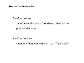
Time series – realization of a stochastic process {Xt} is a stochastic time series if each component takes a value according to a certain probability distribution function. A time series model specifies the joint distribution of the sequence of random variables.
Stochastic properties of the process STATIONARITY System does not change its properties in time Well-developed analytical methods of signal analysis and stochastic processes
WHEN A STOCHASTIC PROCESS IS STATIONARY? • {Xt} is a strictly stationary time series if • (X1,...,Xn)=d (X1+h,...,Xn+h), • where n1, h – integer, =d means distribution equality • Properties: • The random variables are identically distributed. • An idependent identically distributed (iid) sequence is strictly stationary.
Weak stationarity • {Xt} is a weakly stationary time series if • EXt = and Var(Xt)=2are independent of time t • Cov(Xs, Xr) depends on (s-r) only, independent of t. • Properties:E(Xt2) is time-invariant.
Quantitative method for stationarity Reverse Arrangement Test Weak stationarity: Testing if E(Xt2) is time-invariant
Quantile line method • A quantile of order , 0 1, is such a value k(t) that probability of the series taking value less than k(t) at time t equals . • P{Xt k(t)}= • PROPERTIES: • Lines parallel to the time axis stationarity • Lines parallel to each other, not to the time axis constant variance, a variable mean (or median) • Lines not parallel to each other a variable variance (or scale parameter)
Quantile lines of the raw time series Nonstationarity with a variable mean and variance
Methods for nonstationary time series • Trend removal • Segmentation of the series • Specific analytical methods (e.g. ambiguity function, variograms for autocorrelation function)
Trend estimation • Polynomial (or other, e.g. log) estimation and removal • Filters, e.g. moving average filter, FIR, IIR filters • Differencing
Xt = mt + Yt + st random noise seasonal component Stochastic process trend Seasonal modelsClassical decomposition model
Detrended series P. J. Brockwell, R. A. Davis, Introduction to Time Series and Forecasting, Springer, 1987
Range of correlations • Independent data (e.g. WN) • Short-range correlations • Long-range correlations (correlated or anti-correlated structure)
Short-range correlations • Markov processes (e.g. ionic channel conformational transition) • ARMA (ARIMA) linear processes • Nonlinear processes (e.g. GARCH process)
ARMA (ARIMA) models Time series is an ARMA(p,q) process if Xt isstationary and if for every t: Xt1Xt-1 ... pXt-p=Zt+1Zt-1+...+ pZt-p where Zt represents white noise with mean 0 andvariance 2 Left side of the equation represents Autoregresive AR(p) part,and right side Moving Average MA(q) component. The polynomials (1- 1z-...- pzp)cannot have (1+ 1z+...+ pzq) commonfactors.
Examples The range of MA component estimated by ACF (the lag number within Bartlett’s limits ), the range of AR component by PACF Confidence band is
Exponential decay of ACF MA(1)sample ACF AR(1)
Stationary processes with long memory • Qualitative features • Relatively long periods with high or low level of observation values • In short periods there seems to be cycles and local trends. Looking at long series – no particular cycles or persisting trends • Overall the series looks stationary
Stationary processes with long memory • Quantitative features • The variance of the sample mean decays to zero at a slower rate. Instead of there is • The sample autocorrelation function decays to zero in a power-law manner instead of exponentially • Similarly, the periodogram (frequency analysis) shows a power-law
Classical processes with long correlations • Fractional ARIMA processes (fARIMA) • Self similar processes
ARMA (p,q): ARIMA (p,d,q): fractional ARIMA (p,d,q): fARIMA
Self-similar process A process X={X(t)}t 0 is called self-similar if for some H > 0 H=1 – /2 – self-similarity index, (HR +)
Frequency-domain analysisPeriodogram Periodogram - estimated PSD by a Fourier transform of a sample autocorrelation function. Periodogram of a long memory time series depends on frequency according to power-law relationship (straight line on log-log plot). It means that if one doubles the frequency - PSD diminishes by the same fraction regardless of the frequency
Basic features of self similar process • APPEARANCE. If an amplitude of a self-similar process is rescaled by r H, X (rt) looks like X (t), statistically indistinguishable. • VARIANCE of the signal changes as Var (X(t)) t 2H • CORRELATION - correlated or anticorrelated structuring • H=0.5 no memory • H>0.5 long memory • H<0.5 antipersistent long correlations – „short memory” • PERIODOGRAM - power-law dependance on frequency
NileExample J. Beran, Statistics for long-memory processes, Chapman and Hall, 1994
Methods • R/S analysis by Hurst • DFA – Detrended Fluctuation Analysis • Exponent-based (correlogram, periodogram of the residuals) : H=1 – /2 • other (for appropriate PDFs, e.g. Orey index)
Hurst exponent – the algorithm A series with N elements is divided into shorter series – n elements each
Gaussian noise • A series n (n=1,...,N) of uncorrelated and random variables • Each n - Gaussian distribution N(0,) • Brownianmotion • A sum of Gaussian white-noise sequence yn(Bm)= • n(Bm)= n1/2 Fractional Brownian motions (fBm) n(fBm) nH
Fractional Brownian motions (fBm) X={X(t)}t 0 is a nonstationary Gaussian process with mean zero and an autocovariance function: FractionalGaussiannoise(fGn) A stationary process of increments in fBm (differences between values separated by some step)
=0.5 Stable distribution (solid), the attraction domain of stable distribution: Burr and Pareto distributions (broken & dotted) Fractional Lévy Stable Motion In the fractional Lévy stable motion (FLSM) the distribution is Lévy‑stable.
Scaling properties of PDF • -stable distributions have scaling properties – a sum of independent and identically distributed random variables maintains the same shape of the distribution. • Similarly as the Gaussian distribution, also a stable distribution (CLT). • Only a few -stable distributions have direct formulas for their probability density function. Usually only the characteristic function is given. The distinctive properties of -stable distributions are their long tails, infinite variance and, in some cases, infinite mean value.
fractional Levy-stable motion fLSMprocess is a self‑similar non-stationary process which can be represented as Z(u) is a symmetric Lévy -stable motion, and is the stability index of stable distribution. The increment process of FLSM is stationary and it is called a fractional stable noise (FSN).
Memory of a self-similar process d = H 1/ For a Gaussian process =2 For d > 0 the memory is long – a long-range persistent process. Otherwise (d < 0) – a long-range antipersistent process („short memory”). The time series looks very rough
Summary • Time series can be deterministic or stochastic. Visual distinction not always possible. • Stochastic time series may tested analytically by statistical methods and an appropriate model attributed if the series is stationary. Otherwise a pre-processing needed. • Random data in time series may be correlated. Correlations are called memory. • Independent data (e.g. WN) do not have a memory. Each element assumes a value according to an independent probability density function.