Chapter 16 Analyzing and Forecasting Time-Series Data
Business Statistics. Chapter 16 Analyzing and Forecasting Time-Series Data. Chapter Goals. After completing this chapter, you should be able to: Develop and implement basic forecasting models Identify the components present in a time series Compute and interpret basic index numbers

Chapter 16 Analyzing and Forecasting Time-Series Data
E N D
Presentation Transcript
Business Statistics Chapter 16Analyzing and Forecasting Time-Series Data Tran Van Hoang - hoangtv@ftu.edu.vn - Business Statistics
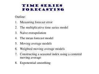
Chapter Goals After completing this chapter, you should be able to: • Develop and implement basic forecasting models • Identify the components present in a time series • Compute and interpret basic index numbers • Use smoothing-based forecasting models, including single and double exponential smoothing • Apply trend-based forecasting models, including linear trend, nonlinear trend, and seasonally adjusted trend Tran Van Hoang - hoangtv@ftu.edu.vn - Business Statistics
The Importance of Forecasting • Governments forecast unemployment, interest rates, and expected revenues from income taxes for policy purposes • Marketing executives forecast demand, sales, and consumer preferences for strategic planning • College administrators forecast enrollments to plan for facilities and for faculty recruitment • Retail stores forecast demand to control inventory levels, hire employees and provide training Tran Van Hoang - hoangtv@ftu.edu.vn - Business Statistics
Time-Series Data • Numerical data obtained at regular time intervals • The time intervals can be annually, quarterly, daily, hourly, etc. • Example: Year: 1999 2000 2001 2002 2003 Sales: 75.3 74.2 78.5 79.7 80.2 Tran Van Hoang - hoangtv@ftu.edu.vn - Business Statistics
Time Series Plot • the vertical axis measures the variable of interest • the horizontal axis corresponds to the time periods A time-series plot is a two-dimensional plot of time series data Tran Van Hoang - hoangtv@ftu.edu.vn - Business Statistics
Time-Series Components Time-Series Trend Component Seasonal Component Cyclical Component Random Component Tran Van Hoang - hoangtv@ftu.edu.vn - Business Statistics
Trend Component • Long-run increase or decrease over time (overall upward or downward movement) • Data taken over a long period of time Sales Upward trend Time Tran Van Hoang - hoangtv@ftu.edu.vn - Business Statistics
Trend Component (continued) • Trend can be upward or downward • Trend can be linear or non-linear Sales Sales Time Time Downward linear trend Upward nonlinear trend Tran Van Hoang - hoangtv@ftu.edu.vn - Business Statistics
Seasonal Component • Short-term regular wave-like patterns • Observed within 1 year • Often monthly or quarterly Sales Summer Winter Fall Spring Time (Quarterly) Tran Van Hoang - hoangtv@ftu.edu.vn - Business Statistics
Cyclical Component • Long-term wave-like patterns • Regularly occur but may vary in length • Often measured peak to peak or trough to trough 1 Cycle Sales Year Tran Van Hoang - hoangtv@ftu.edu.vn - Business Statistics
Random Component • Unpredictable, random, “residual” fluctuations • Due to random variations of • Nature • Accidents or unusual events • “Noise” in the time series Tran Van Hoang - hoangtv@ftu.edu.vn - Business Statistics
Index Numbers • Index numbers allow relative comparisons over time • Index numbers are reported relative to a Base Period Index • Base period index = 100 by definition • Used for an individual item or measurement Tran Van Hoang - hoangtv@ftu.edu.vn - Business Statistics
Index Numbers (continued) • Simple Index number formula: where It = index number at time period t yt = value of the time series at time t y0 = value of the time series in the base period Tran Van Hoang - hoangtv@ftu.edu.vn - Business Statistics
Index Numbers: Example • Company orders from 1995 to 2003: Base Year: Tran Van Hoang - hoangtv@ftu.edu.vn - Business Statistics
Index Numbers: Interpretation • Orders in 1996 were 90% of base year orders • Orders in 2000 were 100% of base year orders (by definition, since 2000 is the base year) • Orders in 2003 were 120% of base year orders Tran Van Hoang - hoangtv@ftu.edu.vn - Business Statistics
Aggregate Price Indexes • An aggregate index is used to measure the rate of change from a base period for a group of items Aggregate Price Indexes Unweighted aggregate price index Weighted aggregate price indexes Paasche Index Laspeyres Index Tran Van Hoang - hoangtv@ftu.edu.vn - Business Statistics
Unweighted Aggregate Price Index • Unweighted aggregate price index formula: where It = unweighted aggregate price index at time t pt = sum of the prices for the group of items at time t p0 = sum of the prices for the group of items in the base period Tran Van Hoang - hoangtv@ftu.edu.vn - Business Statistics
Unweighted Aggregate Price Index Example • Combined expenses in 2004 were 18.8% higher in 2004 than in 2001 Tran Van Hoang - hoangtv@ftu.edu.vn - Business Statistics
Weighted Aggregate Price Indexes • Paasche index • Laspeyres index qt = weighting percentage at q0 = weighting percentage at time t base period pt = price in time period t p0 = price in the base period Tran Van Hoang - hoangtv@ftu.edu.vn - Business Statistics
Commonly Used Index Numbers • Consumer Price Index • Producer Price Index • Stock Market Indexes • Dow Jones Industrial Average • S&P 500 Index • NASDAQ Index Tran Van Hoang - hoangtv@ftu.edu.vn - Business Statistics
Deflating a Time Series • Observed values can be adjusted to base year equivalent • Allows uniform comparison over time • Deflation formula: where = adjusted time series value at time t yt = value of the time series at time t It = index (such as CPI) at time t Tran Van Hoang - hoangtv@ftu.edu.vn - Business Statistics
Deflating a Time Series: Example • Which movie made more money (in real terms)? (Total Gross $ = Total domestic gross ticket receipts in $millions) Tran Van Hoang - hoangtv@ftu.edu.vn - Business Statistics
Deflating a Time Series: Example (continued) • GWTW made about twice as much as Star Wars, and about 4 times as much as Titanic when measured in equivalent dollars Tran Van Hoang - hoangtv@ftu.edu.vn - Business Statistics
Trend-Based Forecasting • Estimate a trend line using regression analysis • Use time (t) as the independent variable: Tran Van Hoang - hoangtv@ftu.edu.vn - Business Statistics
Trend-Based Forecasting (continued) • The linear trend model is: Tran Van Hoang - hoangtv@ftu.edu.vn - Business Statistics
Trend-Based Forecasting (continued) • Forecast for time period 7: Tran Van Hoang - hoangtv@ftu.edu.vn - Business Statistics
Comparing Forecast Values to Actual Data • The forecast error or residual is the difference between the actual value in time t and the forecast value in time t: • Error in time t: Tran Van Hoang - hoangtv@ftu.edu.vn - Business Statistics
Two common Measures of Fit • Measures of fit are used to gauge how well the forecasts match the actual values MSE (mean squared error) • Average squared difference between yt and Ft MAD (mean absolute deviation) • Average absolute value of difference between yt and Ft • Less sensitive to extreme values Tran Van Hoang - hoangtv@ftu.edu.vn - Business Statistics
MSE vs. MAD Mean Square Error Mean Absolute Deviation where: yt = Actual value at time t Ft = Predicted value at time t n = Number of time periods Tran Van Hoang - hoangtv@ftu.edu.vn - Business Statistics
Autocorrelation (continued) • Autocorrelation is correlation of the error terms (residuals) over time • Here, residuals show a cyclic pattern, not random • Violates the regression assumption that residuals are random and independent Tran Van Hoang - hoangtv@ftu.edu.vn - Business Statistics
Testing for Autocorrelation • The Durbin-Watson Statistic is used to test for autocorrelation H0: ρ = 0 (residuals are not correlated) HA: ρ≠ 0 (autocorrelation is present) Durbin-Watson test statistic: Tran Van Hoang - hoangtv@ftu.edu.vn - Business Statistics
Testing for Positive Autocorrelation H0: ρ = 0 (positive autocorrelation does not exist) HA: ρ> 0 (positive autocorrelation is present) • Calculate the Durbin-Watson test statistic = d • (The Durbin-Watson Statistic can be found using PHStat or Minitab) • Find the values dL and dU from the Durbin-Watson table • (for sample size n and number of independent variables p) Decision rule: reject H0 if d < dL Reject H0 Inconclusive Do not reject H0 0 dL dU 2 Tran Van Hoang - hoangtv@ftu.edu.vn - Business Statistics
Testing for Positive Autocorrelation (continued) • Example with n = 25: Excel/PHStat output: Tran Van Hoang - hoangtv@ftu.edu.vn - Business Statistics
Testing for Positive Autocorrelation (continued) • Here, n = 25 and there is one independent variable • Using the Durbin-Watson table, dL = 1.29 and dU = 1.45 • d = 1.00494 < dL = 1.29, soreject H0 and conclude that significant positive autocorrelation exists • Therefore the linear model is not the appropriate model to forecast sales Decision:reject H0 since d = 1.00494 < dL Reject H0 Inconclusive Do not reject H0 0 dL=1.29 dU=1.45 2 Tran Van Hoang - hoangtv@ftu.edu.vn - Business Statistics
Nonlinear Trend Forecasting • A nonlinear regression model can be used when the time series exhibits a nonlinear trend • One form of a nonlinear model: • Compare R2 and sε to that of linear model to see if this is an improvement • Can try other functional forms to get best fit Tran Van Hoang - hoangtv@ftu.edu.vn - Business Statistics
Multiplicative Time-Series Model • Used primarily for forecasting • Allows consideration of seasonal variation • Observed value in time series is the product of components where Tt = Trend value at time t St = Seasonal value at time t Ct = Cyclical value at time t It = Irregular (random) value at time t Tran Van Hoang - hoangtv@ftu.edu.vn - Business Statistics
Finding Seasonal Indexes Ratio-to-moving average method: • Begin by removing the seasonal and irregular components (St and It), leaving the trend and cyclical components (Tt and Ct) • To do this, we need moving averages Moving Average: averages of consecutive time series values Tran Van Hoang - hoangtv@ftu.edu.vn - Business Statistics
Moving Averages • Used for smoothing • Series of arithmetic means over time • Result dependent upon choice of L (length of period for computing means) • To smooth out seasonal variation, L should be equal to the number of seasons • For quarterly data, L = 4 • For monthly data, L = 12 Tran Van Hoang - hoangtv@ftu.edu.vn - Business Statistics
Moving Averages (continued) • Example: Four-quarter moving average • First average: • Second average: • etc… Tran Van Hoang - hoangtv@ftu.edu.vn - Business Statistics
Seasonal Data … … Tran Van Hoang - hoangtv@ftu.edu.vn - Business Statistics
Calculating Moving Averages • Each moving average is for a consecutive block of 4 quarters etc… Tran Van Hoang - hoangtv@ftu.edu.vn - Business Statistics
Centered Moving Averages • Average periods of 2.5 or 3.5 don’t match the original quarters, so we average two consecutive moving averages to get centered moving averages etc… Tran Van Hoang - hoangtv@ftu.edu.vn - Business Statistics
Calculating the Ratio-to-Moving Average • Now estimate the St x It value • Divide the actual sales value by the centered moving average for that quarter • Ratio-to-Moving Average formula: Tran Van Hoang - hoangtv@ftu.edu.vn - Business Statistics
Calculating Seasonal Indexes Tran Van Hoang - hoangtv@ftu.edu.vn - Business Statistics
Calculating Seasonal Indexes (continued) Average all of the Fall values to get Fall’s seasonal index Fall Fall Do the same for the other three seasons to get the other seasonal indexes Fall Tran Van Hoang - hoangtv@ftu.edu.vn - Business Statistics
Interpreting Seasonal Indexes • Suppose we get these seasonal indexes: • Interpretation: Spring sales average 82.5% of the annual average sales Summer sales are 31.0% higher than the annual average sales etc… = 4.000 -- four seasons, so must sum to 4 Tran Van Hoang - hoangtv@ftu.edu.vn - Business Statistics
Deseasonalizing • The data is deseasonalized by dividing the observed value by its seasonal index • This smooths the data by removing seasonal variation Tran Van Hoang - hoangtv@ftu.edu.vn - Business Statistics
Deseasonalizing (continued) etc… Tran Van Hoang - hoangtv@ftu.edu.vn - Business Statistics
Unseasonalized vs. Seasonalized Tran Van Hoang - hoangtv@ftu.edu.vn - Business Statistics
Forecasting Using Smoothing Methods Exponential Smoothing Methods Single Exponential Smoothing Double Exponential Smoothing Tran Van Hoang - hoangtv@ftu.edu.vn - Business Statistics