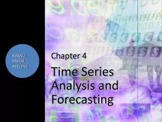
Chapter 4 Time Series Analysis and Forecasting

1. KVANLI PAVUR KEELING Chapter 4Time Series Analysis and Forecasting

2. Chapter Objectives • At the completion of this chapter, you should be able to: ∙ Deseasonalize a time series by first calculating the seasonal indexes ∙ Discuss the nature of additive and multiplicative seasonality ∙ Estimate the trend, cyclical and noise components ∙ Forecast a time series containing trend ∙ Calculate price indexes, including a Laspeyres and Paasche index

3. What is a Time Series? • A time series consists of a variable (such as Sales) recorded across time • Example: tYearSales (millions of $) 1 1985 1.7 2 1986 2.4 3 1987 2.8 4 1988 3.4 . . 22 2006 9.6 23 2007 10.7 This is y1 This is an example of annual data This is y23

4. Time Series Data • Time series data can be: ∙ annual (one value for each year) ∙ quarterly (4 values for each year) ∙ monthly (12 values for each year) • Each time series value is made up of 3 or 4 components. These are: ∙ Trend (TR) ∙ Seasonality (S) ∙ Cyclic (C) ∙ Irregular or noise (I) Monthly or quarterly data only

5. Trend • Trend is the long-term growth or decline in the time series • Trend usually follows a straight line • Examples of linear trend are illustrated in the next two slides

6. Yt Yt t t (a) Increasing trend (b) Decreasing trend Linear Trends

7. 11.0 – 10.0 – 9.0 – 8.0 – 7.0 – 6.0 – 5.0 – 4.0 – 3.0 – 2.0 – 1.0 – Trend Number of employees (thousands) | 2000 | 2001 | 2002 | 2003 | 2004 | 2005 | 2006 | 2007 t Employees Example We’ll take a closer look at this example in the slides to follow

8. Curvilinear Trend • Trend can also be curvilinear • Curvilinear trend is also called quadratic trend • Curvilinear trend is demonstrated in the following three slides • In this chapter, we will pay little attention to curvilinear trend • The macros will assume that trend is linear

9. Yt Yt t t (b) (a) Examples of Curvilinear Trend

10. Yt Yt t t (d) (c) Examples of Curvilinear Trend

11. 300 – 200 – 100 – Power consumption (million kwh) | 1998 | 1999 | 2000 | 2001 | 2002 | 2003 | 2004 | 2005 | 2006 | 2007 t (time) An Illustration of Curvilinear Trend The increase in power consumption slows down over time and the trend is not linear Figure 4.1

12. Seasonality • Seasonality is predictable variation within a year • For example, sales are always high in December • Seasonality only exists for monthly or quarterly data • Two types of seasonal variation ∙ Additive seasonality ∙ Multiplicative seasonality • Seasonal variation will be discussed later in this chapter ∙ Usually the case ∙ Assumed in the Excel macros

13. Cyclical Variation • Cyclical variation is nonseasonal movement about the trend • The next slide illustrates a time series containing cyclical movement (corporate taxes paid by a textile company over a 25-year period) • This time series does not exhibit a trend (long-term upward or downward growth)

14. 4.0 – 3.5 – 3.0 – 2.5 – 2.0 – 1.5 – 1.0 – Corporate taxes (millions of dollars) 1 2 3 | 1980 | 1990 | 2000 | 2005 Textile Example

15. Irregular Activity • Engineers refer to this as “noise” • This is what is left over after measuring the seasonal, trend, and cyclic activity

16. Combining the Components • If the seasonality is assumed to be additive, each yt is the sum of its four components yt = St+TRt + Ct+ It • If the seasonality is assumed to be multiplicative, each yt is the product of its four components yt = St ∙ TRt ∙ Ct ∙ It The seasonal component (St) is omitted for annual data Multiplicative seasonality is the usual situation and assumed in the Excel macros

17. Capturing the Trend • We will illustrate this using annual data which has no seasonality This is the trend line

18. Finding the Trend Line • The equation of the trend line is yt= b0+ b1t • b0 is called the intercept (and is fairly boring) • b1 is called the slope (and is pretty interesting) • The calculations necessary to find the slope and intercept are shown on the next slide

19. Example in Section 2 • ytis the number of employees (in thousands) for eight years • t ytt∙yt 1 1.1 1.1 2 2.4 4.8 3 4.6 13.8 . . 8 11.289.6 48.3 276.3 Let A = the sum of the time series values So, A = 48.3 Let B = the sum of the right-hand column So, B = 276.3 Let T = the number of time periods. So, T = 8

20. Equation of the Trend Line • First, find the slope: • Next, find the intercept:

21. The Example in Section 2 Carry a lot of decimal places The trend line is = -.279 + 1.404t OK to round now

22. Interpreting the Slope • The slope of the trend line is a very interesting value • Here, b1 is 1.404 • Since the number of employees each year (yt) is measured in thousands, then the number of employees in this company is increasing 1,404 (on the average) each year

23. Forecasting – Extending the Trend • If you assume the linear growth or decline as described by the trend line continues for another year, a simple forecast can be obtained from this trend line • For example, what would be your forecast for the year 2008? • This is time period t = 9 • Use this value for t in the trend line equation

24. Forecasting – Extending the Trend • This would be -.279 + 1.404(9) = 12.357 • The forecast for 2008 is 12,357 employees The forecast for 2008 The forecast period sample data

25. Measuring Cyclic Activity – Annual Data • We’ll assume the multiplicative model, where each time series value is the product of its components • Since this is annual data, there is no seasonal component and yt = TRt ∙ Ct ∙ It • The trend line values ( values) contain trend only

26. The Estimated Number of Employees • The estimated number of employees in each time period using the trend line: = -.279 + 1.404(1) = 1.125 = -.279 + 1.404(2) = 2.529 = -.279 + 1.404(3) = 3.933 = -.279 + 1.404(8) = 10.953

27. Measuring Cyclic Activity – Annual Data • By dividing the yt values by the values, you can eliminate the trend components • We’ll call these ratios the cyclic components, even though they contain noise (It) • There is no way to separate out the noise component but it can be reduced when using monthly or quarterly data (illustrated later)

28. tytytyt/yt ^ ^ 1 1.1 1.125 .978 2 2.4 2.529 .949 3 4.6 3.933 1.169 4 5.4 5.337 1.012 5 5.9 6.741 .875 6 8.0 8.145 .982 7 9.7 9.549 1.016 8 11.2 10.953 1.022 Trend and Cyclical Activity Trend activity Cyclical activity

29. Ct 1.15 – 1.10 – 1.05 – 1.00 – .95 – .90 – Start End | 1 | 2 | 3 | 4 | 5 | 6 | 7 | 8 t 2000 2002 2004 2007 Plot of Cyclical Components

30. Yt 11.0 – 10.0 – 9.0 – 8.0 – 7.0 – 6.0 – 5.0 – 4.0 – 3.0 – 2.0 – 1.0 – Actual yt ^ yt = −.279 + 1.404t (trend line) Number of employees (thousands) | 2000 | 2001 | 2002 | 2003 | 2004 | 2005 | 2006 | 2007 t Cyclical Activity

31. Yt Trend 2000 – 1500 – 1000 – 500 – 100 units 100 units Actual time series Units sold 100 units | Winter 2005 | Winter 2006 | Winter 2007 t Additive Seasonal Variation Figure 4.16

32. Yt 700 – 600 – 500 – 400 – 300 – 200 – 100 – TRt = 100 + 20t Sales (tens of thousands of dollars) Estimated sales using trend and seasonality | 1 | 2 | 3 | 4 | 5 | 6 | 7 | 8 | 9 | 10 | 11 | 12 | 13 | 14 | 15 | 16 | 17 | 18 | 19 | 20 t JetskiSales – Additive Seasonality Figure 4.17

33. Yt 2000 – 1500 – 1000 – 500 – 250 units Trend 180 units Units sold Actual time series 100 units | Winter 2005 | Winter 2006 | Winter 2007 t Heat Pump Sales – Multiplicative Seasonality Figure 4.18

34. Yt 700 – 600 – 500 – 400 – 300 – 200 – 100 – TRt = 100 + 20t Sales (tens of thousands of dollars) Estimated sales using trend and seasonality | 1 | 2 | 3 | 4 | 5 | 6 | 7 | 8 | 9 | 10 | 11 | 12 | 13 | 14 | 15 | 16 | 17 | 18 | 19 | 20 t Jetski Sales Multiplicative Season Variation Figure 4.19

35. Procedure with Monthly or Quarterly Data • The Excel macros assume multiplicative seasonality, where yt = St ∙ TRt ∙ Ct ∙ It • Determine the seasonal components (St values) • Deseasonalize the data • Determine the trend components (TRtvalues) using the deseasonalized data • Determine the cyclic components (Ct values) • Determine the irregular (noise) components (It values)