Time Series Forecasting

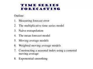
1. Time Series Forecasting • Outline: • Measuring forecast error • The multiplicative time series model • Naïve extrapolation • The mean forecast model • Moving average models • Weighted moving average models • Constructing a seasonal index using a centered moving average • Exponential smoothing

2. Forecast error Forecasting Convenience Store Ice Sales

3. 3 measures of forecast error • Mean absolute deviation • Mean square error • Root mean square error.

4. Actual Predicted Time Average Absolute Error(AAE) is given by: Where Yt is the actual value of variable that we seek to forecast and is the fitted or forecasted value of the variable.

5. Actual Predicted Time Mean Square Error (MSE) is given by: Where Yt is the actual value of variable that we seek to forecast and is the fitted or forecasted value of the variable. • You can think of MSE as the average forecast error. • If we have a perfect forecast, then MSE = 0.

6. Actual Predicted Time Root Mean Square Error (root MSE) is given by: Root MSE is a statistic that is typically is reported by forecasting software applications

7. The Multiplicative Time Series Model • The time path of a variable (such as monthly sales of building materials by supply stores) is produced by the interaction of 4 factors or components. These components are: • The trend component (T) • The seasonal component (S) • The cyclical component (C); and • The irregular component (I)

8. The trend component (T) Trend is the gradual, long-run (or secular) evolution of the variables that we are seeking to forecast.

9. Factors affecting the trend component of a time series • Population changes • Demographic changes. For example, spending for healthcare services is likely to rise due to the aging of the population. Sales of fast food are up due to the secular increase in the female labor force participation rate. • Technological change. Sales of typewriter and vinyl records have trended downward due product innovation. • Changes in consumer tastes and preferences.

10. Linear trends Trend = 10 – 25t Trend = -50 + .8t

11. Non-linear, increasing trend Trend = 10 + .3t + .3t2

12. Non-linear, decreasing trend Trend = 10 - .4t - .4t2

13. The seasonal component (S) • Many series display a regular pattern of variability depending on the time of year. • For example, sales of toys and scotch whiskey peak in December each year. • Ice cream sales are higher in summer months than in winter months. • Car sales tend typically to be strong in May and June and weaker in November and December.

14. The cyclical component (C) • The time path of a series can be influenced by business cycle fluctuations. • For example, we expect housing starts to decline in the contractionary phase of the business cycle. • The same holds true for federal or state tax receipts • The time path of spending for consumer durable goods is also shaped by cyclical forces. • Spending for capital goods is likewise cyclical. • The movie industry has the reputation for being “counter-cyclical”—for example, it flourished during the Depression.

15. The irregular component (I) • The irregular component of the series, sometimes called white noise, is the remaining variability (relative to trend) that cannot be explained by seasonal or cyclical factors. The irregular component is an unexpected, non-recurring factor that affects the series. • For example, hamburger sales plunge due to panic about E-Coli bacteria. • Production of trucks slumps because of a strike at a GM parts plant in Ohio. • Airline slump after 9/11. • A cold snap affects July ice cream sales in upstate NY.

16. If you have a well-designed forecasting model, then forecasting errors should be mainly accounted for by irregular factors

17. The model • Where: • Yt is the value of the time series variable in period t (month t, quarter t, etc.) • Tt trend component of the series in period t • St is the seasonal component of the series in period t • Ct is the cylical component of the series at period t; and • It is the irregular component of the series in period t.

18. The trend component (T) is measured in the units in which the time series itself is measured. So, for example, the trend component for state revenues would be measured in dollars; whereas the trend component for steel production might be measured in tons.

19. The problem: forecast sales of building materials through supply stores for 2000:8 to 2001:7 • The data: • We have monthly data of building material sales through supply stores for the period January 1967 to July 2000 (402 monthly observations). • The data are expressed in millions of current dollars.

20. All data in millions www.economagic.com

21. www.economagic.com

22. Our first step is to estimate thetrend component of our series.This is accomplished using a ordinary least squares, or OLS for short. • OLS is a method of finding the line, or curve, of “best fit.” • The trend function of best fit is the one that minimizes the squared sum of the vertical distances of the sample points (the actual monthly values of building materials sales) from the trend line (fitted values of monthly building materials sales).

23. OLS • Let: • Yt be the actual value of building materials sales in month t; • Let Ŷt be the trend value of building materials sales in month t. The trend function we are seeking satisfies the following condition:

24. Professor Brown has estimated two trend functions—one linear and one non-linear. They are displayed on the the following two slides. • The trend of of building materials sales since 1967 is positive and increasing (non-linear).

25. Trend = -771.28 + 25.79t

26. Trend = 957.77 + 0.11t + .063t2

27. Trend = 957.77 + 0.11t + .063t2

28. Example: Trend value of building material sales for March 81 Note that, for March 1981 t= 169 Trend = 957.77 + 0.11t + .063t2 Thus we have: TrendMar 81= 957.77 +[(.11)(169)] + [(.063)(1692]

29. The Seasonal Index • If you sum the indices for each month, and divide by 12, you get 1.00. • Notice that, on average for the period 1967-2000, July has been the best month for sales of building materials, and February the worst month. • Later, we will show you a simple technique for constructional a seasonal index—a centered moving average.

30. Performing an in-sample forecast of building materials sales • An in-sample forecast means we are forecasting building material sales for those months for which we already have data that have been used to estimate the trend, seasonal, and other components. Comparing forecasted, or fitted values of building material sales with actual time series data gives us an idea of how well this performs. • We will assume that the cyclical index is equal to 1 (Ct = 1). This is a poor assumption since our period contains several business cycle episodes.

31. Let’s give an example how we we use this model to forecast building material sales for a particular month, say, March 1981 again.Recall that t = 169 for this month

32. In-sample forecasts using the multiplicative time series model

33. Residuals for in-sample forecast MSE = 179,288root MSE = $423 million

34. Assumption that Ct = 1 results in substantial in-sample forecast errors Recessionary periods are shaded

35. Forecasting Sales of Building Materials Using the Multiplicative Time Series Model All data in millions