Statistical Forecasting Models
Statistical Forecasting Models. (Lesson - 07). Best Bet to See the Future. Statistical Forecasting Models. Time Series Models : independent variable is time. Moving Average Exponential Smoothening Holt-Winters Model Explanatory Methods : independent variable is one or more factor(s).

Statistical Forecasting Models
E N D
Presentation Transcript
Statistical Forecasting Models (Lesson - 07) Best Bet to See the Future Dr. C. Ertuna
Statistical Forecasting Models • Time Series Models: independent variable is time. • Moving Average • Exponential Smoothening • Holt-Winters Model • Explanatory Methods: independent variable is one or more factor(s). • Regression Dr. C. Ertuna
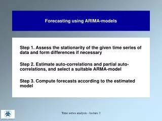
Time Series Models • Statistical Time Series Models are very useful for short range forecasting problems such as weekly sales. • Time series models assume that whatever forces have influenced the variables in question (sales) in the recent past will continue into the near future. Dr. C. Ertuna
Time Series Components A time series can be described by models based on the following components Tt Trend Component St Seasonal Component Ct Cyclical Component It Irregular Component Using these components we can define a time series as the sum of its components or an additive model Alternatively, in other circumstances we might define a time series as the product of its components or a multiplicative model – often represented as a logarithmic model Dr. C. Ertuna
Components of Time Series Data • A linear trend is any long-term increase or decrease in a time series in which the rate of change is relatively constant. • A seasonal component is a pattern that is repeated throughout a time series and has a recurrence period of at most one year. • A cyclical component is a pattern within the time series that repeats itself throughout the time series and has a recurrence period of more than one year. Dr. C. Ertuna
Components of Time Series Data • The irregular (or random) component refers to changes in the time-series data that are unpredictable and cannot be associated with the trend, seasonal, or cyclical components. Dr. C. Ertuna
Stationary Time Series Models Time series with constant mean and variance are called stationary time series. When Trend, Seasonal, or Cyclical effects are not significant then • Moving Average Models and • Exponential Smoothing Models are useful over short time periods. Dr. C. Ertuna
Moving Average Models • Simple Moving Average forecast is computed as the average of the most recent k-observations. • Weighted Moving Average forecast is computed as the weighted average of the most recent k-observations where the most recent observation has the highest weight. Dr. C. Ertuna
Moving Average Models • Simple Moving AverageForecast • Weighted Moving AverageForecast Dr. C. Ertuna
To determine best weights and period (k) we can use forecast accuracy. MSE = Mean Square Error is a good measure for forecast accuracy. RMSE = is the square root of the MSE. Weighted Moving Average Data: Evens - Burglaries Dr. C. Ertuna
Weighted Moving Average • Tools / Solver • Set Target Cell: Cell containing RMSE value • Equal to: Min • By Changing Cells: Cells containing weights • Subject to constraints: Cell containing sum of the weight = 1 • Options / (check) Assume Non-Negativity • Solve ----- Keep Solver Solution ----- OK Dr. C. Ertuna
Best weights for a given “k” (in this case “3”) is determined by solver trough minimizing RMSE. Same procedure could be applied to models with different k’s and the one with lowest RMSE could be considered as the model with best forecasting period. Weighted Moving Average Dr. C. Ertuna
Tools/ Data Analysis / Moving Average Input Range: Observations with title (No time) Output Range: Select next column to the input range and 1-Row below of the first observation Chart misaligns the forecasted values! Forecasted 59th month is aligned with 58th month Moving Average Models Dr. C. Ertuna
Exponential Smoothing Exponential smoothing is a time-series smoothing and forecasting technique that produces an exponentially weighted moving average in which each smoothing calculation or forecast is dependent upon all previously observed values. • The smoothing factor “α” is a value between 0 and 1, where α closer to 1 means more weigh to the recent observations and hence more rapidly changing forecast. Dr. C. Ertuna
Exponential Smoothing Model or where: Ft= Forecast value for period t Yt-1 = Actual value for period t-1 Ft-1 = Forecast value for period t-1 = Alpha (smoothing constant) Dr. C. Ertuna
Exponential Smoothing Model • Tools/ Data Analysis / Exponential Smoothing. • Input Range: Observations with title (No time) • Output Range: Select next column to the input range and first Row of the first observation • Damping Factor: 1-α (not α) Dr. C. Ertuna
To determine best “α” we can use forecast accuracy. MSE = Mean Square Error is a good measure for forecast accuracy. Exponential Smoothing Model Dr. C. Ertuna
Holt-Winters Model The Holt-Winters forecasting model could be used in forecasting trends. Holt-Winters model consists of both an exponentially smoothing component (E, w) and a trend component (T, v) with two different smoothing factors. Dr. C. Ertuna
Holt-Winters Model where: Ft+k= Forecast value k periods from t Yt-1 = Actual value for period t-1 Et-1 = Estimated value for period t-1 Tt = Trend for period t w = Smoothing constant for estimates v = Smoothing factor for trend k = number of periods • E1 and T1 are not defined. • E2 = Y2 • T2 = Y2 – Y1 Dr. C. Ertuna
Holt-Winters Model • E_2 = Y_2 and T_2 = (Y_2-Y_1) • E_12 = $D$1*C14+(1-$D$1)*(D13+E13) • T_12 = $E$1*(D14-D13)+(1-$E$1)*E13 • F_13 = D14+E14 Dr. C. Ertuna
Holt-Winters Model • Set E (smoothing component), T (trend component), and F (forecasted values) columns next to Y (actual observations) in the same sequence • Determine initial “w” and “v” values • Leave E,T &F blanc for the base period (t=1) • Set E2 = Y2 • Set T2 = Y2-Y1Note: (F2 is blanc) Dr. C. Ertuna
Holt-Winters Model • Formulate E3 = w*Y3 + (1-w)*(E2+T2) • Formulate T3 = v*(E3-E2) + (1-v)*T2 • Formulate F3 = E2 + T2 • Copy the formulas down until reaching one cell further than the last observation (Yn). • Compute MSE using Y’s and F’s • Use solver to determine optimal “w” and “v”. Dr. C. Ertuna
Holt-Winters Model Solver set up for Holt Winters: • Target Cell: MSE (min) • Changing Cells: w andv • Constrains: w <= 1 w >= 0 v <= 1 v >= 0 Dr. C. Ertuna
Forecasting with Crystal Ball • CBTools / CB Predictor • [Input Data] Select Range, First Raw, First Column Next • [Data Attribute]Data is in Next • [Method Gallery]Select All Next • [Results]Number of periods to forecast [1] Select Past Forecasts at cell Run periods, etc. Dr. C. Ertuna
Forecasting with Crystal Ball Dr. C. Ertuna
Forecasting with Crystal Ball Dr. C. Ertuna
Performance of a Model Performance of a model is measured byTheil’s U. The Theil's U statistic falls between 0 and1. When U=0,that means that the predictive performance of the model is excellant and when U=1 then it means that the forecasting performance is not better than just using the last actual observation as a forecast. Dr. C. Ertuna
Theil’sU versus RMSE The difference between RMSE (or MAD or MAPE) and Theil’s U is that the formars are measure of ‘fit’; measuring how well model fits to the historical data. The Theil's Uon the other hand measures how well the model predicts against a ‘naive’ model. A forecast in a naive model is done by repeating the most recent value of the variable as the next forecasted value. Dr. C. Ertuna
Choosing Forecasting Model The forecasting model should be the one with lowest Theil’s U. If the best Theil’s U model is not the same as the best RMSE model then you need to run CB again by checking only the best Theil’s U model to obtain forecasted value. P.S. CB uses forecasting value of the lowest RMSE model (best model according CB)! Dr. C. Ertuna
Determining Performance Theil’s U determins the forecasting performance of the model. The interpretation in daily language is as follows: Interpret (1- Thei’l U) 1.00 – 0.80 High (strong) forecasting power 0.80 – 0.60 Moderately high forecasting power 0.60 – 0.40 Moderate forecasting power 0.40 – 0.20 Weak forecasting power 0.20 – 0.00 Very weak forecasting power Dr. C. Ertuna
Regression or Time Series Forecast Here is the guiding principlewhen to apply Regression and when to apply Time Series Forecast. • As some thing changes (one or more independent variables) how does another thing (dependent variable) changeis an issue of directional relationshipFor directional relationships we can use regression. • If the independent variable is TIME (as time changes how does a variable change)Then we can use either regression or time series forecasting models Dr. C. Ertuna
Explanatory Methods Simple Linear Regression Model: The simplest inferential forecasting model is the simple linear regression model, where time (t) is the independent variable and the least square line is used to forecast the future values of Yt. Dr. C. Ertuna
Regression in Forecasting Trends where: Yt = Value of trend at time t 0 = Intercept of the trend line 1 = Slope of the trend line t = Time (t = 1, 2, . . . ) Dr. C. Ertuna
Regression in Forecasting Seasonality • Many time series have distinct seasonal pattern. (For example room sales are usually highest around summer periods.) • Multiple regression models can be used to forecast a time series with seasonal components. • The use of dummy variables for seasonality is common. • Dummy variables needed = total number of seasonality –1 • For example: Quarterly Seasonal: 3 Dummies are needed, Monthly Seasonal: 11 Dummies needed, etc. • The load of each seasonal variable (dummy) is compared to the one which is hidden in intercept. Dr. C. Ertuna
Regression in Forecasting Seasonality where: Q1 = 1 , if quarter is 1, = 0 otherwise Q2 = 1 , if quarter is 2, = 0 otherwise Q3 = 1 , if quarter is 3, = 0 otherwise 2 = the load of Q1 above Q4 0 = the overall intercept + the load of Q4 t = Time (t = 1, 2, . . . ) Dr. C. Ertuna
Seasonal Regression E(Y_Q1) = -10801.6 + 5.52 * Year.1 + 8.06 E(Y_Q2) = -10801.6 + 5.52 * Year.2 + -3.50 E(Y_Q3) = -10801.6 + 5.52 * Year.3 + 5.51 E(Y_Q4) = -10801.6 + 5.52 * Year.4 Dr. C. Ertuna
Next Lesson (Lesson - 09) Introduction to Optimization Dr. C. Ertuna
![Statistical Forecasting [Part 2]](https://cdn0.slideserve.com/1092555/statistical-forecasting-part-2-dt.jpg)


![Statistical Forecasting [Part 1]](https://cdn3.slideserve.com/6737421/statistical-forecasting-part-1-dt.jpg)