Download

1 / 85
850 likes | 1.02k Vues
Using the Particle Filter Approach to Building Partial Correspondences between Shapes. Rolf Lakaemper, Marc Sobel Temple University, Philadelphia,PA,USA. Part I: Motivation. The Goal: Finding correspondences between feature-points in two (similar) shapes. The Motivation:

E N D
Using the Particle Filter Approach to Building Partial Correspondences between Shapes Rolf Lakaemper, Marc Sobel Temple University, Philadelphia,PA,USA
Part I: Motivation
The Goal: Finding correspondences between feature-points in two (similar) shapes
The Motivation: Shape recognition. Classically divided into three steps: • Finding correspondences (this talk) • Alignment • Shape Similarity
We want to handle partialcorrespondences between arbitrary point sets based on local descriptors and certain global constraints. This includes but is not limited to…
The simplest case: Closed boundaries vs. Closed boundaries
Advanced: Closed polygons vs. polygons representing parts
More advanced: Partial matching of unordered 2D point sets
…and unordered 3D point sets Bad example due to insufficient constraints. Later we’ll see how to improve it.
These tasks can be described as an optimization problem. They will only differ in the way the global constraints are defined. We will present a Particle Filter (PF) based solution unifying these problems. The PF system is able to learn properties of the global constraints.
General Approach Single Particle (configuration of established correspondences) Local Constraints GC update rule Particle Filtering Global Constraints (GC) Task PF Framework
Part II: Illustration of the Approach using the simple example of correspondences between closed boundary curves
The example data: boundary polygons • Each boundary curve is uniformly sub sampled • Each shape is represented by an ordered set of boundary points
II.A Local Constraints
For each boundary point we computelocal feature descriptors, eventually leading to a local correspondence matrix. This matrix describes the local constraints. Single Particle (configuration of established correspondences) Local Constraints GC update rule Particle Filtering Global Constraints (GC)
Computation of Local Feature Descriptors. As an example we use • Centroid Distance • Curvature Remark: research is not about optimal, new and fancy local descriptors. On the contrary: for several reasons we use relatively weak descriptors
Centroid Distance (normalized, average dist. = 1) Relative distance to center of polygon (mean of vertices) Extendable to parts • Curvature e.g. turn angle
Using each descriptor independently, we compute the correspondence probability between all pairs of points. • The correspondence is computed in a symmetric way: • How likely is it that pi in shape1 corresponds to qk in shape2 relative to all points in shape2 AND • How likely is it that qk in shape2 corresponds to pi in shape1 relative to all points in shape1
Example: Centroid Distance • Compute correspondence matrix MD1 = [md1ij] ui = centroid distance of point i in shape1 vj = centroid distance of point j in shape2 Gσ = Gauss Distribution with standard deviation σ • Row normalize MD1
MD1 described the correspondence probability of a point in shape1 to a point in shape2. To find the correspondence probability shape2 to shape1, compute MD2 (column normalized):
Finally, the correspondence matrix MD is the element wise product of MD1 and MD2: MD = MD1 .* MD2
The correspondence matrix MC using curvature is computed accordingly • The final localcorrespondence matrix is the joint probability of both features L = MD .* MC
Correspondences MC MD MC.*MD
MC MD MC.*MD
Conclusion about L: • L defines a probability Pc over the set C of correspondences • L(S1,S2) = LT (S2,S1). This means L is order independent with respect to S1, S2. This of course does NOT necessarily mean that L is symmetric. • L is symmetric S1=S2 • just as a note: M(S1,S1) (the self similarity matrix) is not necessarily diagonal dominant (see ‘device’ example).
L defines the weights of single correspondences. Finding the optimal correspondence configuration is the task of finding a certain path in L under certain constraints. In our example, the constraints are: • One to one correspondences only • Order preservation The following section will formalize the optimization problem.
II.B Correspondence as optimization problem
Definitions: • A groupingg in the set G of all groupings is a configuration of correspondences. • Global constraints restrict the search space for our optimization process to G- (a subset of G), the admissible groupings • Using L (=Pc), we define a weight function W over G
We formulate the correspondence problem as one of choosing the grouping, g^ ∈ G− from the set of admissible groupings, G− with maximal weight or, more specifically: Lemma 1: the optimal grouping is complete
The optimization problem could typically be solved using dynamic programming We want to use particle filters to solve the correspondence problem Reason: particle filters provide a less restricted framework, which enables us to extend the system to solve more general and complex recognition problems (parts, inner structures, 3D shapes)
II.C Using Particle Filters to solve the optimization problem
Particle Filters Single Particle (configuration of established correspondences) Local Constraints GC update rule Particle Filtering Global Constraints (GC)
Some general remarks: Particle Filtering, e.g. in contrast to the deterministic Dynamic Programming, is a statistical approach. It does not guarantee an optimal (but only a near optimal) solution.
But: the weight matrix is built from non-precise local descriptors. Hence a precise, optimal solution does not necessarily make sense anyway.
The goal of particle filters (PF) is to estimate the posterior distribution over the entire search space using discrete distributions (constructed dynamically at each of a number of different iterations) based on a limited number of particles. For our optimization problem, we are interested in the strongest particle. Whatever dialect of PF is used, they always consist of 2 major steps:
Let’s say we have n particles (hypotheses). Each particle has a ‘weight’. Step 1: Prediction Corresponding to additional information, update each particle and compute its new weight. Step 2: Evaluation Pick n updated particles according to their weights. ‘Better’ particles have a higher chance to survive.
In our example problem, a single particle is a set of order preserving correspondences. Its weight is computed using the weights of the single correspondences.
Prediction: add a new correspondence (order preserving) based on the and compute the new weight. The new correspondence is picked using the distribution defined by the weight matrix L Evaluation: Residual sub sampling. Additionally we use a RECEDE step: every m steps, n correspondences are deleted (m>n). This can be seen as an add on to the update step.
Adding correspondences randomly means: we do not need to know a starting point, we also do not need to know the direction of the path (this is an advantage, though not the main advantage over dynamic programming) • The order constraint decreases the size of the search space rapidly
Updating using the correspondence matrix L as underlying distribution has 2 effects: • Correspondences of high probability are likely to be picked first • Correspondences in indistinct areas of L have a uniform distribution. This problem is automatically solved, since our system prefers particles with a higher number of correspondences.
The main contribution: L is dynamically modified using GLOBAL constraints These constraints are modeled by a global constraint matrix, which is re-built for each particle in each step. The matrix contains real valued elements, weakening the admissibility definition to ‘degree of admissibility’
II.D Global constraints in our example
Adding Global Constraints Single Particle (configuration of established correspondences) Local Constraints GC update rule Particle Filtering Global Constraints (GC)
Finding the optimal global correspondence between two shapes: we want an optimal correspondence configuration based on L AND • We want to maximize the number of correspondences • We want to conserve the point order
We want to find a maximal and order preserving path in M We do NOT know the number of correspondences, the start point or the path direction (Matrix M is a torus, i.e. circular in both dimensions)
An order preserving max. path is a set of correspondences of shape vertices
Order preservation can be formulated in terms of a global constraint matrix with entries {0,1}
The particle selection process operates on the product of the local and global matrix. The strict distinction between local and global constraints will be of use in more advanced applications, which we will see later. Our optimization process operates on a dynamically changing matrix.